Analysis of Clinical Trial Data

In this piece of an experimental project, we will examine factors that could lead to survival in breast cancer patients. Appropriate machine learning algorithm would be deployed to model the dataset using the tidymodels methodology in R.

Introduction

Breast cancer is a disease in which cells in the breast grow out of control. There are different kinds of breast cancer. The kind of breast cancer depends on which cells in the breast turn into cancer. Breast cancer can begin in different parts of the breast. Medical professionals often opined that earlier detection of breast cancer is key to survival.

In this piece of an experimental project, we will examine factors that could lead to survival in breast cancer patients. Appropriate machine learning algorithm would be deployed to model the dataset using the tidymodels methodology in R.

Load Libraries

Code

#if(!require(pacman)) install.packages("pacman")

pacman::p_load(
  tidyverse,
  magrittr,
  reactable,
  ggthemes,
  DescTools,
  tidymodels,
  vip
)

options(scipen = 999, digits = 2)

Load Dataset

Code

# Load datasets

survival_tbl <- read_csv('dataset.csv')

Code

# structure and data types of the fields

glimpse(survival_tbl)

Rows: 120
Columns: 4
$ Age            <dbl> 45, 74, 58, 66, 57, 42, 70, 62, 43, 46, 41, 67, 56, 63,~
$ Operation_year <dbl> 68, 65, 59, 58, 64, 63, 58, 66, 64, 65, 59, 66, 67, 66,~
$ nr_of_nodes    <dbl> 0, 3, 0, 1, 1, 1, 4, 0, 0, 20, 0, 0, 0, 0, 11, 0, 8, 8,~
$ survival       <dbl> 1, 2, 1, 1, 2, 1, 2, 1, 2, 2, 1, 1, 1, 1, 1, 1, 1, 1, 2~

Data Wrangling

Convert the dependent variable survival to factor.

Code

# Convert the dependent variable `survival` to factor

survival_tbl %<>%
  mutate(survival = if_else(survival == 1, "The patient survived 5 years or longer", "The patient died within 5 years"),
         survival = as.factor(survival))

Exploratory Data Analysis of the Dataset

Code

glimpse(survival_tbl)

Rows: 120
Columns: 4
$ Age            <dbl> 45, 74, 58, 66, 57, 42, 70, 62, 43, 46, 41, 67, 56, 63,~
$ Operation_year <dbl> 68, 65, 59, 58, 64, 63, 58, 66, 64, 65, 59, 66, 67, 66,~
$ nr_of_nodes    <dbl> 0, 3, 0, 1, 1, 1, 4, 0, 0, 20, 0, 0, 0, 0, 11, 0, 8, 8,~
$ survival       <fct> The patient survived 5 years or longer, The patient die~

Code

reactable(survival_tbl, searchable = TRUE, filterable = TRUE, sortable = TRUE, pagination = TRUE)

Code

# brief data summary

summary(survival_tbl)

      Age     Operation_year  nr_of_nodes
 Min.   :30   Min.   :58     Min.   : 0  
 1st Qu.:44   1st Qu.:60     1st Qu.: 0  
 Median :54   Median :63     Median : 0  
 Mean   :53   Mean   :63     Mean   : 4  
 3rd Qu.:62   3rd Qu.:66     3rd Qu.: 3  
 Max.   :78   Max.   :69     Max.   :46  
                                   survival 
 The patient died within 5 years       :29  
 The patient survived 5 years or longer:91  
                                            
                                            
                                            
                                            

Code

# detailed summary

Desc(survival_tbl)

------------------------------------------------------------------------------ 
Describe survival_tbl (tbl_df, tbl, data.frame):

data frame: 120 obs. of  4 variables
        120 complete cases (100.0%)

  Nr  ColName         Class    NAs  Levels                                  
  1   Age             numeric  .                                            
  2   Operation_year  numeric  .                                            
  3   nr_of_nodes     numeric  .                                            
  4   survival        factor   .    (2): 1-The patient died within 5 years, 
                                    2-The patient survived 5 years or longer


------------------------------------------------------------------------------ 
1 - Age (numeric)

  length       n    NAs  unique     0s   mean  meanCI'
     120     120      0      44      0  53.02   50.95
          100.0%   0.0%           0.0%          55.10
                                                     
     .05     .10    .25  median    .75    .90     .95
   36.90   38.00  43.75   53.50  62.00  69.10   71.05
                                                     
   range      sd  vcoef     mad    IQR   skew    kurt
   48.00   11.50   0.22   13.34  18.25   0.05   -0.90
                                                     
lowest : 30.0 (2), 31.0, 33.0, 34.0, 35.0
highest: 72.0, 73.0, 74.0 (2), 76.0, 78.0

' 95%-CI (classic)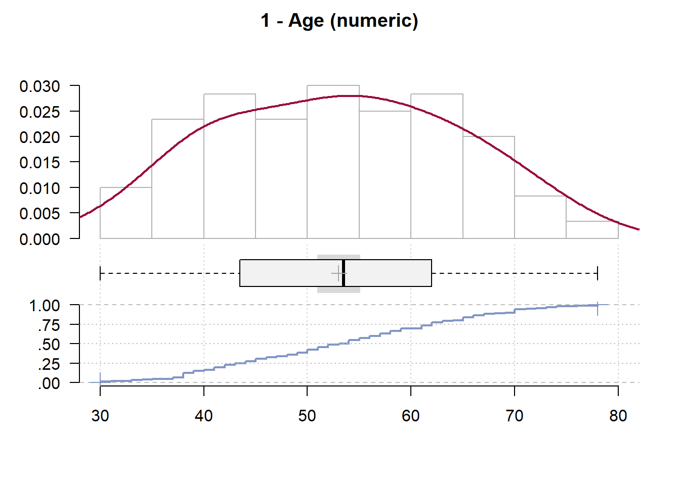

------------------------------------------------------------------------------ 
2 - Operation_year (numeric)

  length       n    NAs  unique     0s   mean  meanCI'
     120     120      0      12      0  63.10   62.48
          100.0%   0.0%           0.0%          63.72
                                                     
     .05     .10    .25  median    .75    .90     .95
   58.00   58.00  60.00   63.00  66.00  67.00   68.05
                                                     
   range      sd  vcoef     mad    IQR   skew    kurt
   11.00    3.41   0.05    4.45   6.00  -0.01   -1.26
                                                     

    value  freq   perc  cumfreq  cumperc
1      58    14  11.7%       14    11.7%
2      59    13  10.8%       27    22.5%
3      60     7   5.8%       34    28.3%
4      61     9   7.5%       43    35.8%
5      62    10   8.3%       53    44.2%
6      63     8   6.7%       61    50.8%
7      64    14  11.7%       75    62.5%
8      65     8   6.7%       83    69.2%
9      66    12  10.0%       95    79.2%
10     67    14  11.7%      109    90.8%
11     68     5   4.2%      114    95.0%
12     69     6   5.0%      120   100.0%

' 95%-CI (classic)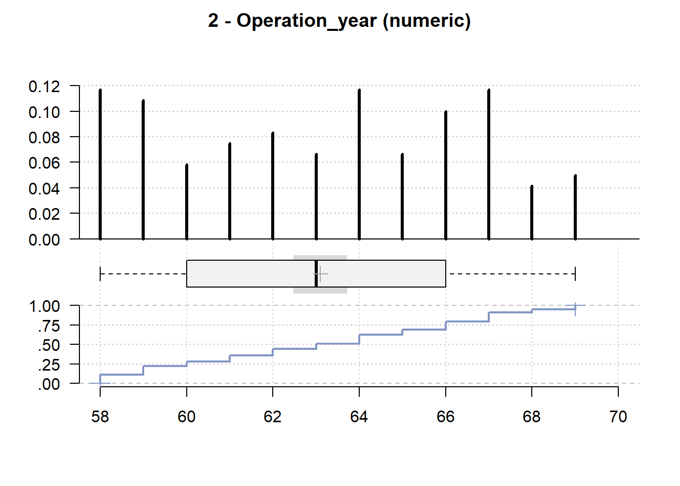

------------------------------------------------------------------------------ 
3 - nr_of_nodes (numeric)

  length       n    NAs  unique     0s   mean  meanCI'
     120     120      0      20     60   3.57    2.31
          100.0%   0.0%          50.0%           4.82
                                                     
     .05     .10    .25  median    .75    .90     .95
    0.00    0.00   0.00    0.50   3.00  13.00   15.20
                                                     
   range      sd  vcoef     mad    IQR   skew    kurt
   46.00    6.96   1.95    0.74   3.00   3.26   13.42
                                                     
lowest : 0.0 (60), 1.0 (14), 2.0 (8), 3.0 (9), 4.0 (3)
highest: 19.0 (2), 20.0, 22.0, 35.0, 46.0

heap(?): remarkable frequency (50.0%) for the mode(s) (= 0)

' 95%-CI (classic)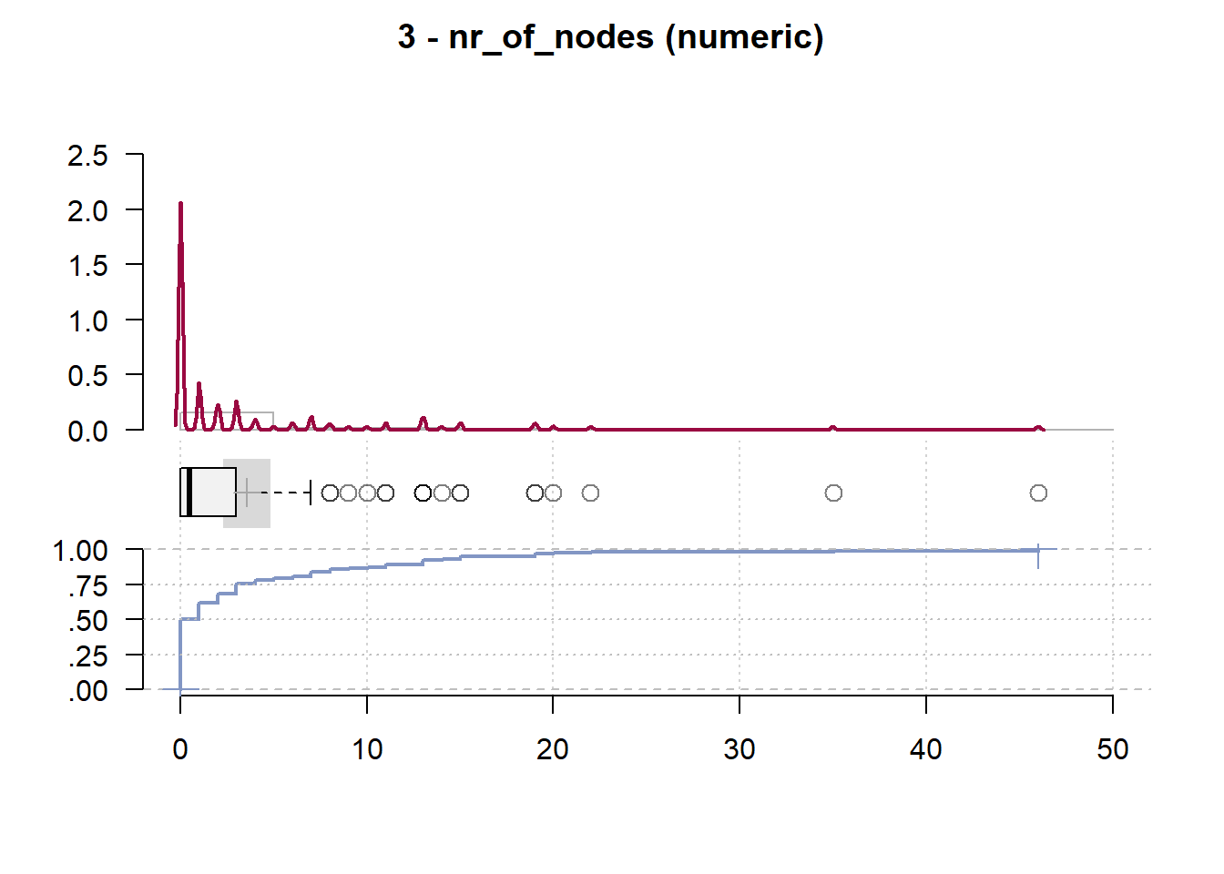

------------------------------------------------------------------------------ 
4 - survival (factor - dichotomous)

  length      n    NAs unique
     120    120      0      2
         100.0%   0.0%       

                                        freq   perc  lci.95  uci.95'
The patient died within 5 years           29  24.2%   17.4%   32.6%
The patient survived 5 years or longer    91  75.8%   67.4%   82.6%

' 95%-CI (Wilson)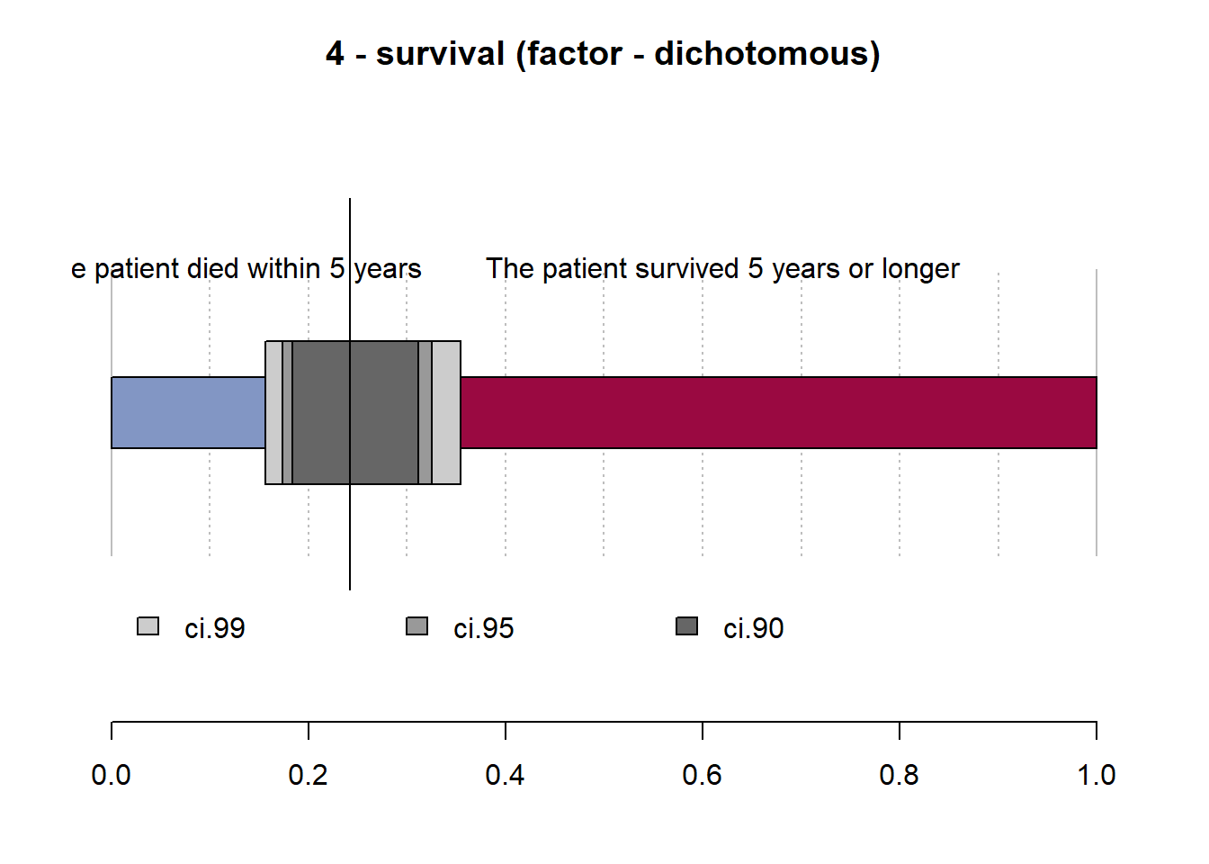

Code

# Survival Distribution

survival_tbl %>% 
  group_by(survival) %>%
  summarise(Freq = n()) %>% 
  mutate(prop = Freq/sum(Freq)) %>% 
  filter(Freq != 0) %>% 
  
  ggplot(mapping = aes(x = 2, y = prop, fill = survival))+
  geom_bar(width = 1, color = "white", stat = "identity") +
  xlim(0.5, 2.5) +
  coord_polar(theta = "y", start = 0) +
  theme_void() +
  scale_y_continuous(labels = scales::percent) +
  geom_text(aes(label = paste0(round(prop*100, 1), "%")), size = 4, position = position_stack(vjust = 0.5)) +
  scale_fill_manual(values = c("#fc0394","#03adfc")) +
  #theme(axis.text.x = element_text(angle = 90), legend.position = "top")+
  labs(title = "Patient survival distribution",
       x = "",
       y = "",
       fill = "") +
  theme(legend.position = "top") +
   theme(title = element_text(family = "Sans", face = "bold", size = 16))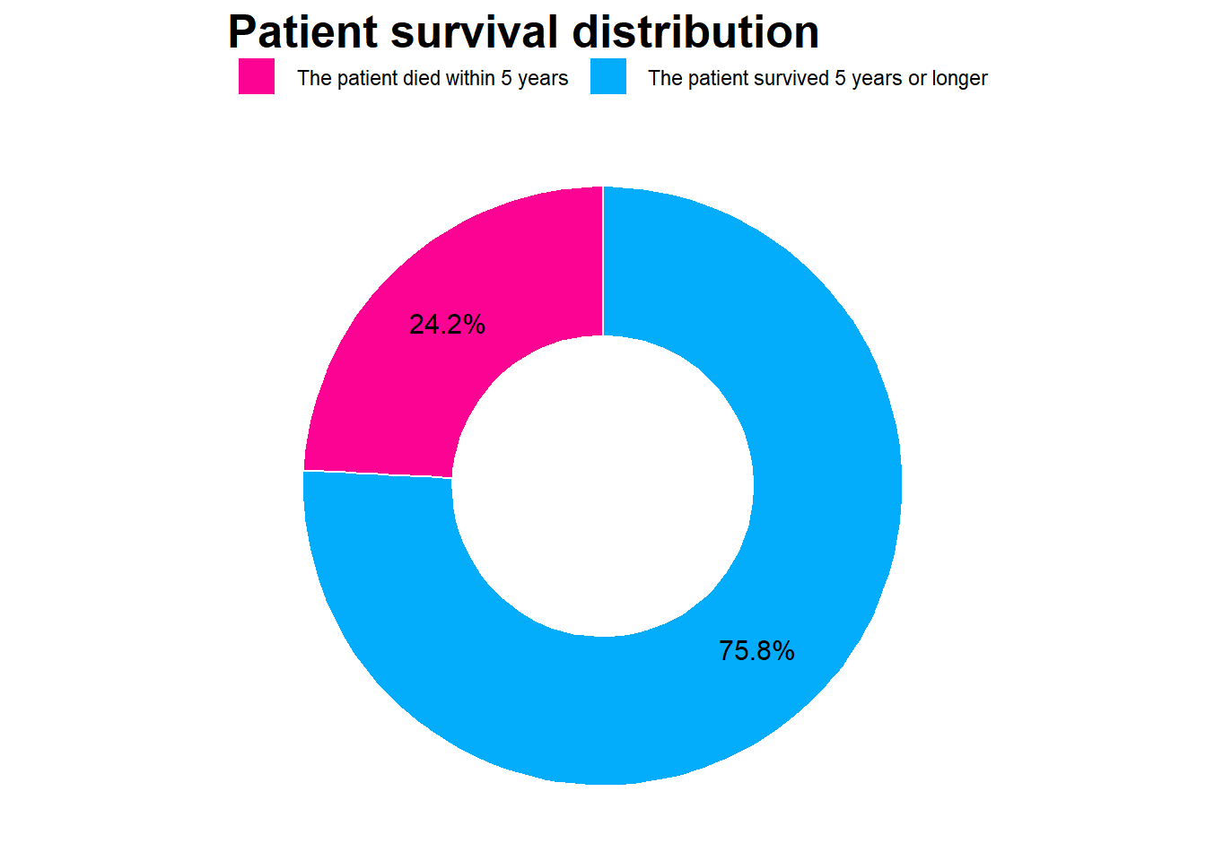

Code

# Age Distribution

ggplot(survival_tbl, aes(Age)) +
  geom_histogram(fill = "steelblue", color = "white") +
  labs(title = 'Patient age distribution',
       x = "Age",
       y = "Frequency",
       fill = "") +
   theme(title = element_text(family = "Sans", face = "bold", size = 16)) +
  theme_clean()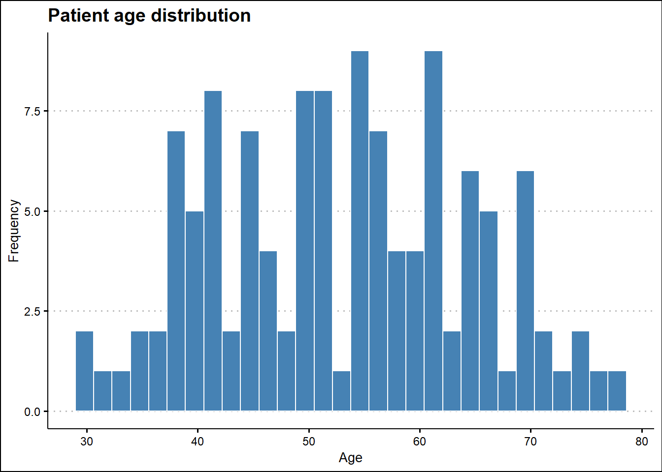

Code

# Distribution of positive auxiliary nodes detected

ggplot(survival_tbl, aes(nr_of_nodes)) +
  geom_histogram(fill = "steelblue", color = "white") +
  labs(title = 'Distribution of positive auxiliary nodes',
       x = "# of Auxiliary Nodes",
       y = "Frequency",
       fill = "") +
   theme(title = element_text(family = "Sans", face = "bold", size = 16)) +
  theme_clean()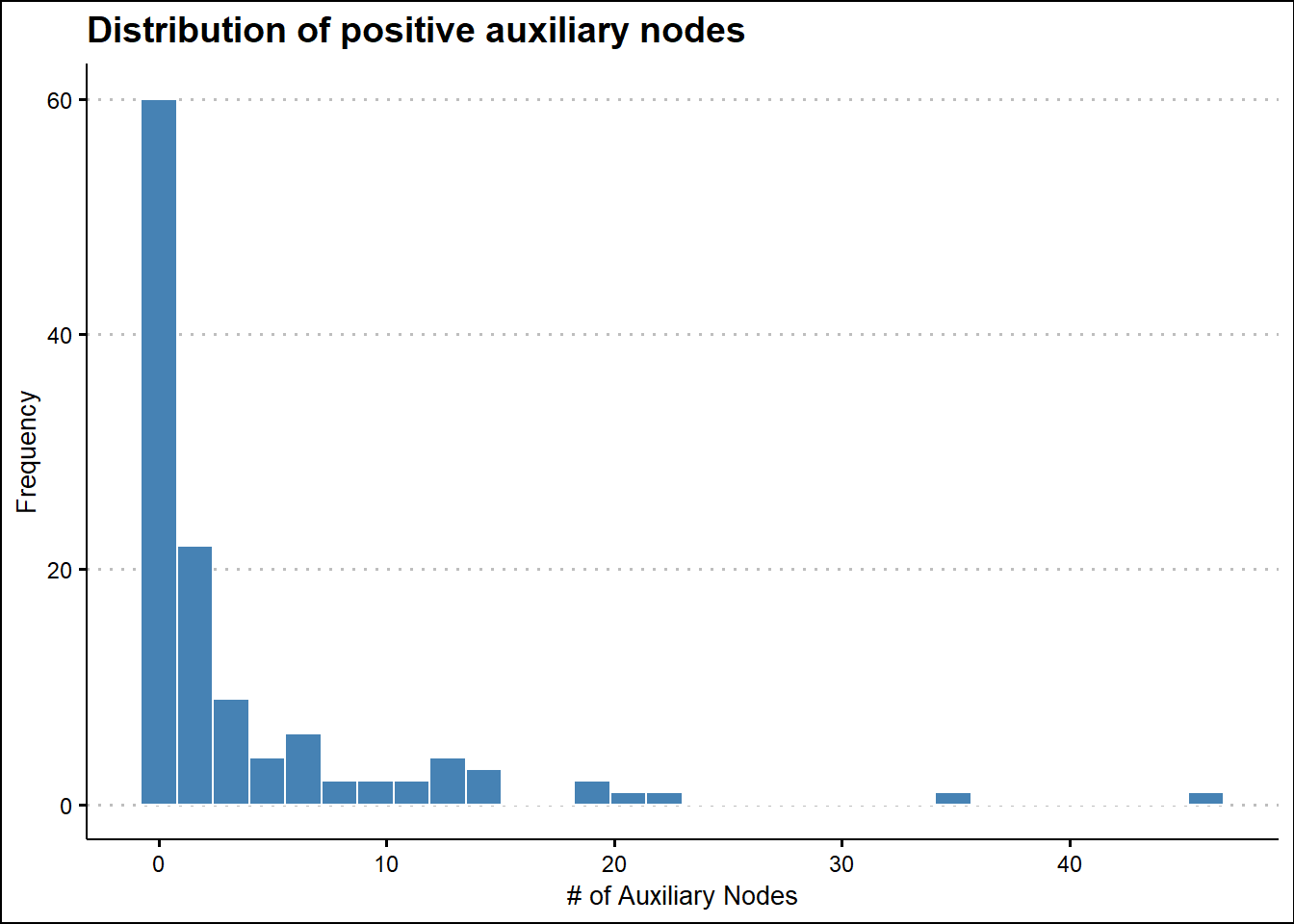

Code

# Counts of surgery performed yearly

survival_tbl %>% 
  mutate(Operation_year = paste0("19", Operation_year)) %>% 
  group_by(Operation_year) %>% 
  summarise(Count = n()) %>% 
  ggplot(aes(x = Operation_year, y = Count)) +
  geom_bar(stat = "identity", width = 0.5, fill = "steelblue", color = "white") +
  labs(title = 'Count of surgery performed yearly',
       x = "Year of operation") +
  theme(title = element_text(family = "Sans", face = "bold", size = 16),
        axis.title = element_text(family = "sans", size = 10, face = "plain")) +
  theme_clean() +
  scale_y_continuous(labels = scales::comma) +
  geom_text(aes(label = Count), size = 4)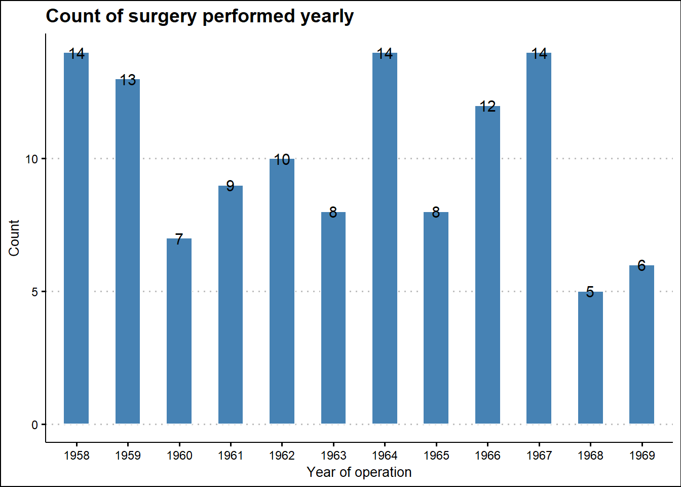

Modelling

Data Quality

Check dataframe for NAs

Code

any(is.na(survival_tbl))

[1] FALSE

• No NA is found. The dataset is complete without any missing values.

Code

# split data to train and test set

set.seed(1234)

split <- survival_tbl %>% 
  initial_split(prop = 0.75, strata = survival) # 75% training set | 25% testing set

df_train <- split %>% 
  training()

df_test <- split %>% 
  testing()

Model Recipe

Code

rec <- recipe(survival ~ ., data = df_train)

# add preprocessing

prepro <- rec %>% 
  step_normalize(all_numeric_predictors()) %>% 
  prep()

prepro

Define the model with parsnip

Code

## Logistic Regression

lr <- logistic_reg(
  mode = "classification"
) %>% 
  set_engine("glm")

Define models workflow

Code

## Logistic Regression

lr_wf <- workflow() %>% 
  add_recipe(prepro) %>% 
  add_model(lr)

Model Fitting

Code

set.seed(1234)

## Logistic Regression

lr_wf %>% 
  fit(df_train) %>% 
 tidy()

# A tibble: 4 x 5
  term           estimate std.error statistic    p.value
  <chr>             <dbl>     <dbl>     <dbl>      <dbl>
1 (Intercept)      1.29       0.283     4.57  0.00000483
2 Age             -0.147      0.286    -0.515 0.606     
3 Operation_year  -0.0605     0.278    -0.218 0.828     
4 nr_of_nodes     -1.09       0.324    -3.37  0.000745  

Obtaining Predictions

Code

set.seed(1234)

## Logistic Regression

lr_pred <- lr_wf %>% 
  fit(df_train) %>% 
  predict(df_test) %>% 
  bind_cols(df_test)

Evaluating model performance

• kap: Kappa
• sens: Sensitivity
• spec: Specificity
• f_meas: F1
• mcc: Matthews correlation coefficient

Logistic Regression

Code

lr_pred %>% 
  conf_mat(truth = survival, estimate = .pred_class) %>% 
  autoplot(type = "heatmap")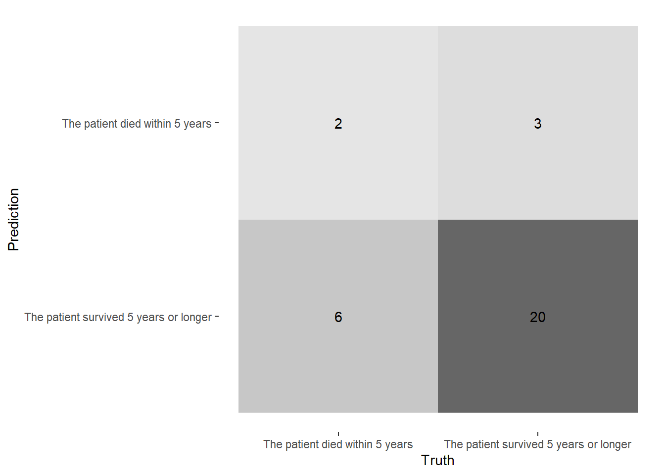

Code

lr_pred %>% 
  conf_mat(truth = survival, estimate = .pred_class) %>% 
  summary()

# A tibble: 13 x 3
   .metric              .estimator .estimate
   <chr>                <chr>          <dbl>
 1 accuracy             binary         0.710
 2 kap                  binary         0.136
 3 sens                 binary         0.25 
 4 spec                 binary         0.870
 5 ppv                  binary         0.4  
 6 npv                  binary         0.769
 7 mcc                  binary         0.142
 8 j_index              binary         0.120
 9 bal_accuracy         binary         0.560
10 detection_prevalence binary         0.161
11 precision            binary         0.4  
12 recall               binary         0.25 
13 f_meas               binary         0.308

Roc Curve and AUC estimate

Code

prob_preds <- lr_wf %>% 
  fit(df_train) %>% 
  predict(df_test, type = "prob") %>% 
  bind_cols(df_test)


threshold_df <- prob_preds %>% 
  roc_curve(truth = survival, estimate = `.pred_The patient survived 5 years or longer`)

threshold_df %>% 
  autoplot()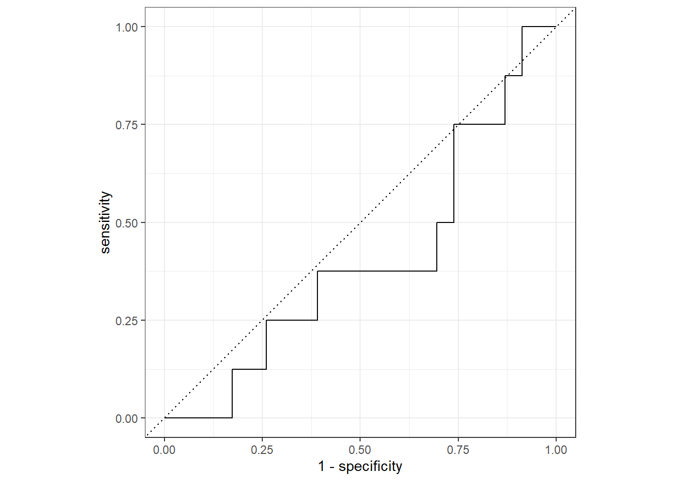

Code

roc_auc(prob_preds, truth = survival, estimate = `.pred_The patient survived 5 years or longer`)

# A tibble: 1 x 3
  .metric .estimator .estimate
  <chr>   <chr>          <dbl>
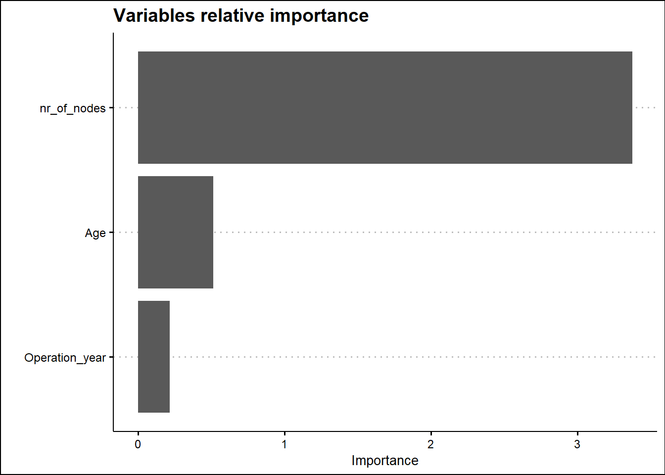
1 roc_auc binary         0.402

Variable Importance Plot

Relative variable importance plot

Code

final_lr_model <-
  lr_wf %>%
  fit(data = df_train)

final_lr_model

== Workflow [trained] ==========================================================
Preprocessor: Recipe
Model: logistic_reg()

-- Preprocessor ----------------------------------------------------------------
1 Recipe Step

* step_normalize()

-- Model -----------------------------------------------------------------------

Call:  stats::glm(formula = ..y ~ ., family = stats::binomial, data = data)

Coefficients:
   (Intercept)             Age  Operation_year     nr_of_nodes  
        1.2929         -0.1472         -0.0605         -1.0910  

Degrees of Freedom: 88 Total (i.e. Null);  85 Residual
Null Deviance:      97 
Residual Deviance: 81   AIC: 89

Code

final_lr_model %>% 
  extract_fit_parsnip() %>% 
  tidy()

# A tibble: 4 x 5
  term           estimate std.error statistic    p.value
  <chr>             <dbl>     <dbl>     <dbl>      <dbl>
1 (Intercept)      1.29       0.283     4.57  0.00000483
2 Age             -0.147      0.286    -0.515 0.606     
3 Operation_year  -0.0605     0.278    -0.218 0.828     
4 nr_of_nodes     -1.09       0.324    -3.37  0.000745  

Code

## variable importance plot

final_lr_model %>%
  extract_fit_parsnip() %>%
  vip() +
  labs(title = 'Variables relative importance',
       x = "") +
  theme(title = element_text(family = "Sans", face = "bold", size = 16),
        axis.title = element_text(family = "sans", size = 10, face = "plain")) +
  theme_clean() +
  scale_y_continuous(labels = scales::comma)