Telco Customer Churn

Focused customer retention programs

Machine Learning

Tidymodels

Clinical Data

Classification

Predictive Analytics

Tidyverse

This experimental project addresses the customer churn in a telecommunication company. Different classification models are considered in the modeling section using the tidymodels methodology in R.

Author

Olumide Oyalola

Published

March 3, 2023

Introduction

The ultimate goals of any business enterprise is to maximize profit, minimize cost, ensure efficiency in service delivery among others. In order to achieve this, the business ensures that the estimate customer base is maintained over time. In terms of cost, it’s cost effective to maintain an existing customer than to acquire a new one. To this effect, every business enterprise ensures that the churn rate to minimized and also endeavor to identify factors that could be responsible for customer churn and addresses them accordingly.

This experimental project addresses the customer churn in a telecommunication company.

Different classification models are considered in the modeling section using the tidymodels methodology in R.

Load Libraries and Datasets

Code

library(tidyverse)
library(magrittr)
library(reactable)
library(naniar)
library(ggthemes)
library(ggcorrplot)
library(DescTools)
library(tidymodels)
library(zoo)

Code

# Load datasets

telco_df <- read_csv('WA_Fn-UseC_-Telco-Customer-Churn.csv')

Code

# structure and data types of the fields

glimpse(telco_df)

Rows: 7,043
Columns: 21
$ customerID       <chr> "7590-VHVEG", "5575-GNVDE", "3668-QPYBK", "7795-CFOCW~
$ gender           <chr> "Female", "Male", "Male", "Male", "Female", "Female",~
$ SeniorCitizen    <dbl> 0, 0, 0, 0, 0, 0, 0, 0, 0, 0, 0, 0, 0, 0, 0, 0, 0, 0,~
$ Partner          <chr> "Yes", "No", "No", "No", "No", "No", "No", "No", "Yes~
$ Dependents       <chr> "No", "No", "No", "No", "No", "No", "Yes", "No", "No"~
$ tenure           <dbl> 1, 34, 2, 45, 2, 8, 22, 10, 28, 62, 13, 16, 58, 49, 2~
$ PhoneService     <chr> "No", "Yes", "Yes", "No", "Yes", "Yes", "Yes", "No", ~
$ MultipleLines    <chr> "No phone service", "No", "No", "No phone service", "~
$ InternetService  <chr> "DSL", "DSL", "DSL", "DSL", "Fiber optic", "Fiber opt~
$ OnlineSecurity   <chr> "No", "Yes", "Yes", "Yes", "No", "No", "No", "Yes", "~
$ OnlineBackup     <chr> "Yes", "No", "Yes", "No", "No", "No", "Yes", "No", "N~
$ DeviceProtection <chr> "No", "Yes", "No", "Yes", "No", "Yes", "No", "No", "Y~
$ TechSupport      <chr> "No", "No", "No", "Yes", "No", "No", "No", "No", "Yes~
$ StreamingTV      <chr> "No", "No", "No", "No", "No", "Yes", "Yes", "No", "Ye~
$ StreamingMovies  <chr> "No", "No", "No", "No", "No", "Yes", "No", "No", "Yes~
$ Contract         <chr> "Month-to-month", "One year", "Month-to-month", "One ~
$ PaperlessBilling <chr> "Yes", "No", "Yes", "No", "Yes", "Yes", "Yes", "No", ~
$ PaymentMethod    <chr> "Electronic check", "Mailed check", "Mailed check", "~
$ MonthlyCharges   <dbl> 29.85, 56.95, 53.85, 42.30, 70.70, 99.65, 89.10, 29.7~
$ TotalCharges     <dbl> 29.85, 1889.50, 108.15, 1840.75, 151.65, 820.50, 1949~
$ Churn            <chr> "No", "No", "Yes", "No", "Yes", "Yes", "No", "No", "Y~

Data Wrangling

Convert character typed data to factor except the customerID field

Code

# convert character typed data to factor except the customerID

telco_df %<>%
  select_if(is.character) %>% 
  mutate(across(c(where(is.character), -c(customerID)), as.factor))

Exploratory Data Analysis of the Dataset

Code

glimpse(telco_df)

Rows: 7,043
Columns: 17
$ customerID       <chr> "7590-VHVEG", "5575-GNVDE", "3668-QPYBK", "7795-CFOCW~
$ gender           <fct> Female, Male, Male, Male, Female, Female, Male, Femal~
$ Partner          <fct> Yes, No, No, No, No, No, No, No, Yes, No, Yes, No, Ye~
$ Dependents       <fct> No, No, No, No, No, No, Yes, No, No, Yes, Yes, No, No~
$ PhoneService     <fct> No, Yes, Yes, No, Yes, Yes, Yes, No, Yes, Yes, Yes, Y~
$ MultipleLines    <fct> No phone service, No, No, No phone service, No, Yes, ~
$ InternetService  <fct> DSL, DSL, DSL, DSL, Fiber optic, Fiber optic, Fiber o~
$ OnlineSecurity   <fct> No, Yes, Yes, Yes, No, No, No, Yes, No, Yes, Yes, No ~
$ OnlineBackup     <fct> Yes, No, Yes, No, No, No, Yes, No, No, Yes, No, No in~
$ DeviceProtection <fct> No, Yes, No, Yes, No, Yes, No, No, Yes, No, No, No in~
$ TechSupport      <fct> No, No, No, Yes, No, No, No, No, Yes, No, No, No inte~
$ StreamingTV      <fct> No, No, No, No, No, Yes, Yes, No, Yes, No, No, No int~
$ StreamingMovies  <fct> No, No, No, No, No, Yes, No, No, Yes, No, No, No inte~
$ Contract         <fct> Month-to-month, One year, Month-to-month, One year, M~
$ PaperlessBilling <fct> Yes, No, Yes, No, Yes, Yes, Yes, No, Yes, No, Yes, No~
$ PaymentMethod    <fct> Electronic check, Mailed check, Mailed check, Bank tr~
$ Churn            <fct> No, No, Yes, No, Yes, Yes, No, No, Yes, No, No, No, N~

Code

reactable(telco_df, searchable = TRUE, filterable = TRUE, sortable = TRUE, pagination = TRUE)

Code

# brief data summary

summary(telco_df)

  customerID           gender     Partner    Dependents PhoneService
 Length:7043        Female:3488   No :3641   No :4933   No : 682    
 Class :character   Male  :3555   Yes:3402   Yes:2110   Yes:6361    
 Mode  :character                                                   
                                                                    
          MultipleLines     InternetService             OnlineSecurity
 No              :3390   DSL        :2421   No                 :3498  
 No phone service: 682   Fiber optic:3096   No internet service:1526  
 Yes             :2971   No         :1526   Yes                :2019  
                                                                      
              OnlineBackup             DeviceProtection
 No                 :3088   No                 :3095   
 No internet service:1526   No internet service:1526   
 Yes                :2429   Yes                :2422   
                                                       
              TechSupport                StreamingTV  
 No                 :3473   No                 :2810  
 No internet service:1526   No internet service:1526  
 Yes                :2044   Yes                :2707  
                                                      
            StreamingMovies           Contract    PaperlessBilling
 No                 :2785   Month-to-month:3875   No :2872        
 No internet service:1526   One year      :1473   Yes:4171        
 Yes                :2732   Two year      :1695                   
                                                                  
                   PaymentMethod  Churn     
 Bank transfer (automatic):1544   No :5174  
 Credit card (automatic)  :1522   Yes:1869  
 Electronic check         :2365             
 Mailed check             :1612

Code

# detailed summary

Desc(telco_df)

------------------------------------------------------------------------------ 
Describe telco_df (tbl_df, tbl, data.frame):

data frame: 7043 obs. of  17 variables
        7043 complete cases (100.0%)

  Nr  ColName           Class      NAs  Levels                            
  1   customerID        character  .                                      
  2   gender            factor     .    (2): 1-Female, 2-Male             
  3   Partner           factor     .    (2): 1-No, 2-Yes                  
  4   Dependents        factor     .    (2): 1-No, 2-Yes                  
  5   PhoneService      factor     .    (2): 1-No, 2-Yes                  
  6   MultipleLines     factor     .    (3): 1-No, 2-No phone service,    
                                        3-Yes                             
  7   InternetService   factor     .    (3): 1-DSL, 2-Fiber optic, 3-No   
  8   OnlineSecurity    factor     .    (3): 1-No, 2-No internet service, 
                                        3-Yes                             
  9   OnlineBackup      factor     .    (3): 1-No, 2-No internet service, 
                                        3-Yes                             
  10  DeviceProtection  factor     .    (3): 1-No, 2-No internet service, 
                                        3-Yes                             
  11  TechSupport       factor     .    (3): 1-No, 2-No internet service, 
                                        3-Yes                             
  12  StreamingTV       factor     .    (3): 1-No, 2-No internet service, 
                                        3-Yes                             
  13  StreamingMovies   factor     .    (3): 1-No, 2-No internet service, 
                                        3-Yes                             
  14  Contract          factor     .    (3): 1-Month-to-month, 2-One year,
                                        3-Two year                        
  15  PaperlessBilling  factor     .    (2): 1-No, 2-Yes                  
  16  PaymentMethod     factor     .    (4): 1-Bank transfer (automatic), 
                                        2-Credit card (automatic),        
                                        3-Electronic check, 4-Mailed check
  17  Churn             factor     .    (2): 1-No, 2-Yes                  


------------------------------------------------------------------------------ 
1 - customerID (character)

  length      n    NAs unique levels  dupes
   7'043  7'043      0  7'043  7'043      n
         100.0%   0.0%                     

         level  freq  perc  cumfreq  cumperc
1   0002-ORFBO     1  0.0%        1     0.0%
2   0003-MKNFE     1  0.0%        2     0.0%
3   0004-TLHLJ     1  0.0%        3     0.0%
4   0011-IGKFF     1  0.0%        4     0.1%
5   0013-EXCHZ     1  0.0%        5     0.1%
6   0013-MHZWF     1  0.0%        6     0.1%
7   0013-SMEOE     1  0.0%        7     0.1%
8   0014-BMAQU     1  0.0%        8     0.1%
9   0015-UOCOJ     1  0.0%        9     0.1%
10  0016-QLJIS     1  0.0%       10     0.1%
11  0017-DINOC     1  0.0%       11     0.2%
12  0017-IUDMW     1  0.0%       12     0.2%
... etc.
 [list output truncated]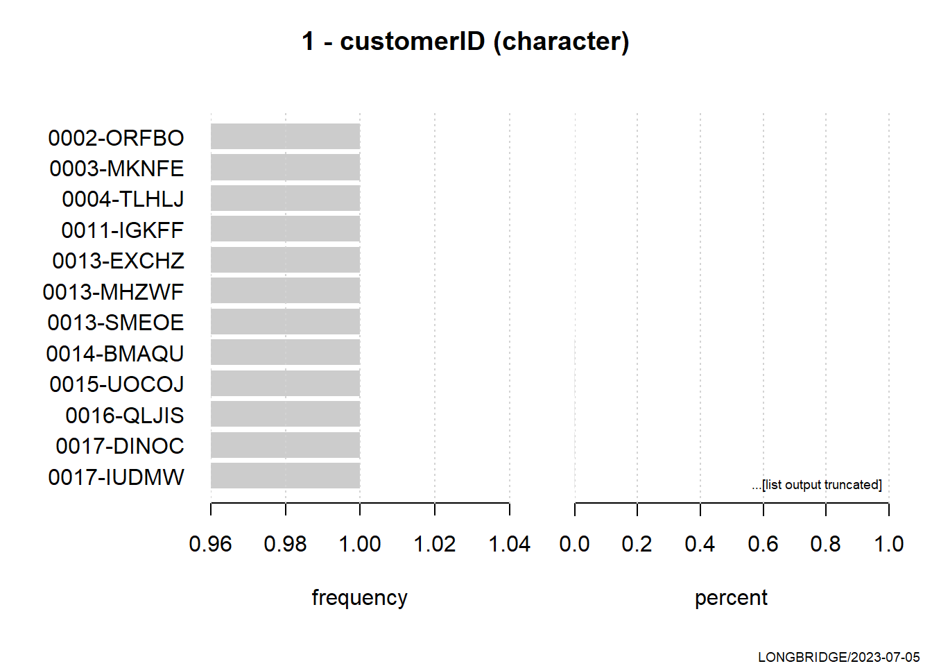

------------------------------------------------------------------------------ 
2 - gender (factor - dichotomous)

  length      n    NAs unique
   7'043  7'043      0      2
         100.0%   0.0%       

         freq   perc  lci.95  uci.95'
Female  3'488  49.5%   48.4%   50.7%
Male    3'555  50.5%   49.3%   51.6%

' 95%-CI (Wilson)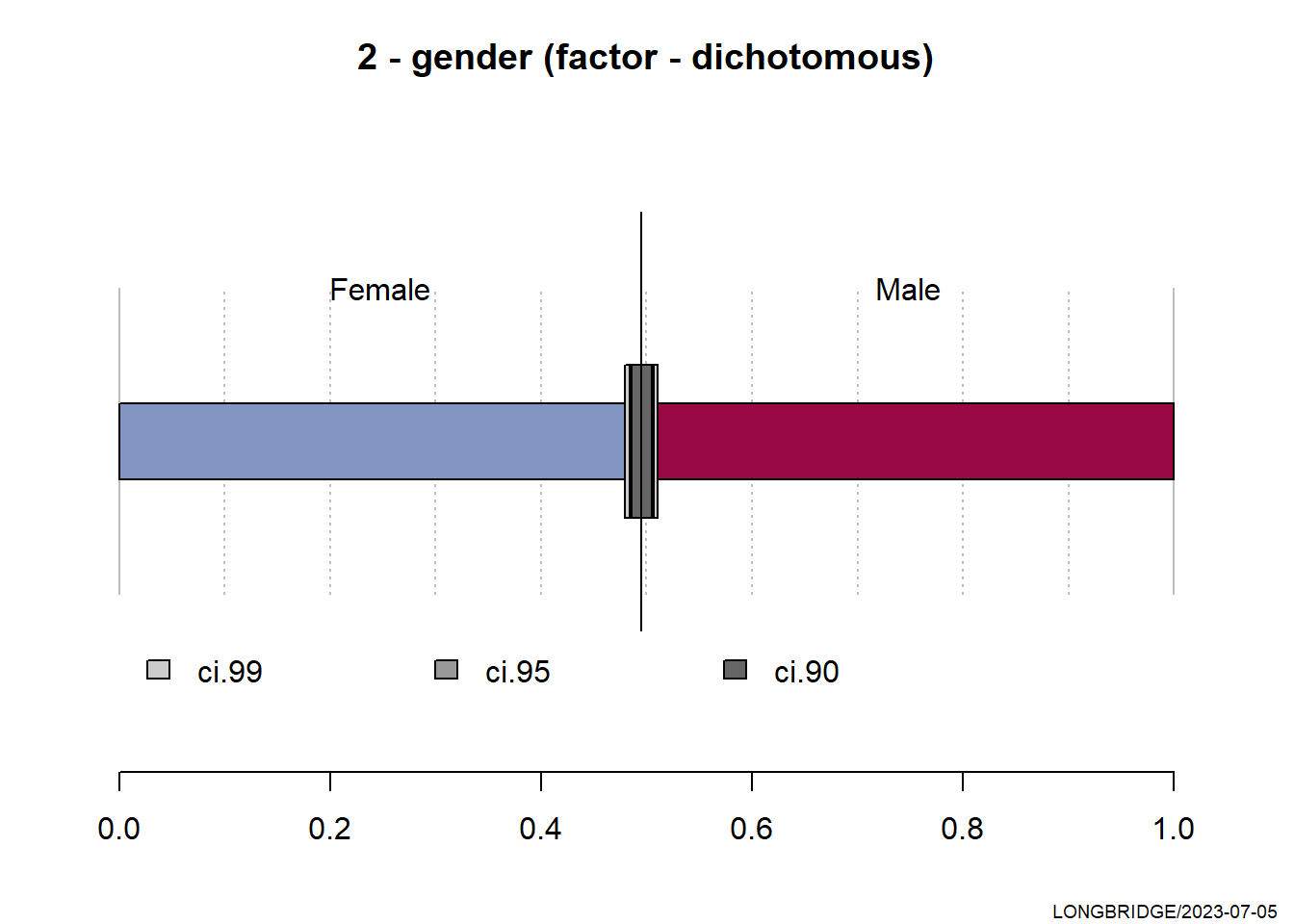

------------------------------------------------------------------------------ 
3 - Partner (factor - dichotomous)

  length      n    NAs unique
   7'043  7'043      0      2
         100.0%   0.0%       

      freq   perc  lci.95  uci.95'
No   3'641  51.7%   50.5%   52.9%
Yes  3'402  48.3%   47.1%   49.5%

' 95%-CI (Wilson)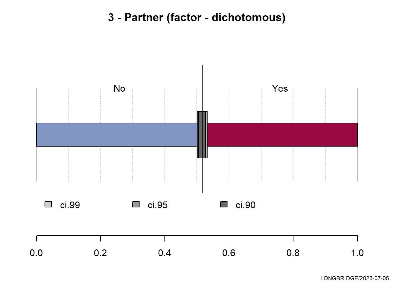

------------------------------------------------------------------------------ 
4 - Dependents (factor - dichotomous)

  length      n    NAs unique
   7'043  7'043      0      2
         100.0%   0.0%       

      freq   perc  lci.95  uci.95'
No   4'933  70.0%   69.0%   71.1%
Yes  2'110  30.0%   28.9%   31.0%

' 95%-CI (Wilson)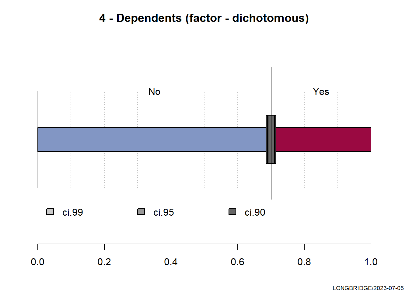

------------------------------------------------------------------------------ 
5 - PhoneService (factor - dichotomous)

  length      n    NAs unique
   7'043  7'043      0      2
         100.0%   0.0%       

      freq   perc  lci.95  uci.95'
No     682   9.7%    9.0%   10.4%
Yes  6'361  90.3%   89.6%   91.0%

' 95%-CI (Wilson)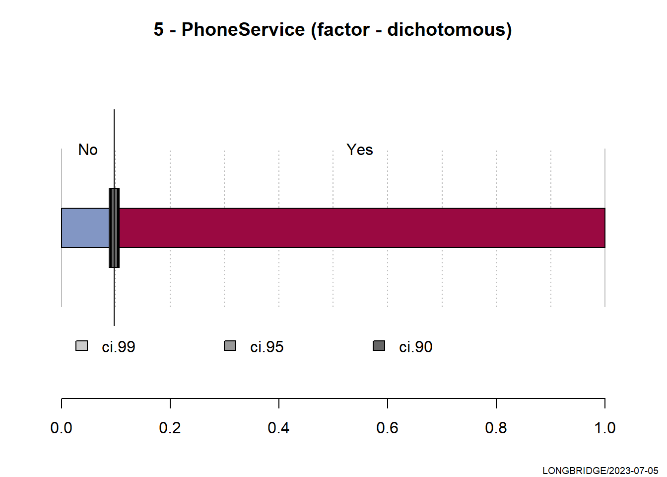

------------------------------------------------------------------------------ 
6 - MultipleLines (factor)

  length      n    NAs unique levels  dupes
   7'043  7'043      0      3      3      y
         100.0%   0.0%                     

              level   freq   perc  cumfreq  cumperc
1                No  3'390  48.1%    3'390    48.1%
2               Yes  2'971  42.2%    6'361    90.3%
3  No phone service    682   9.7%    7'043   100.0%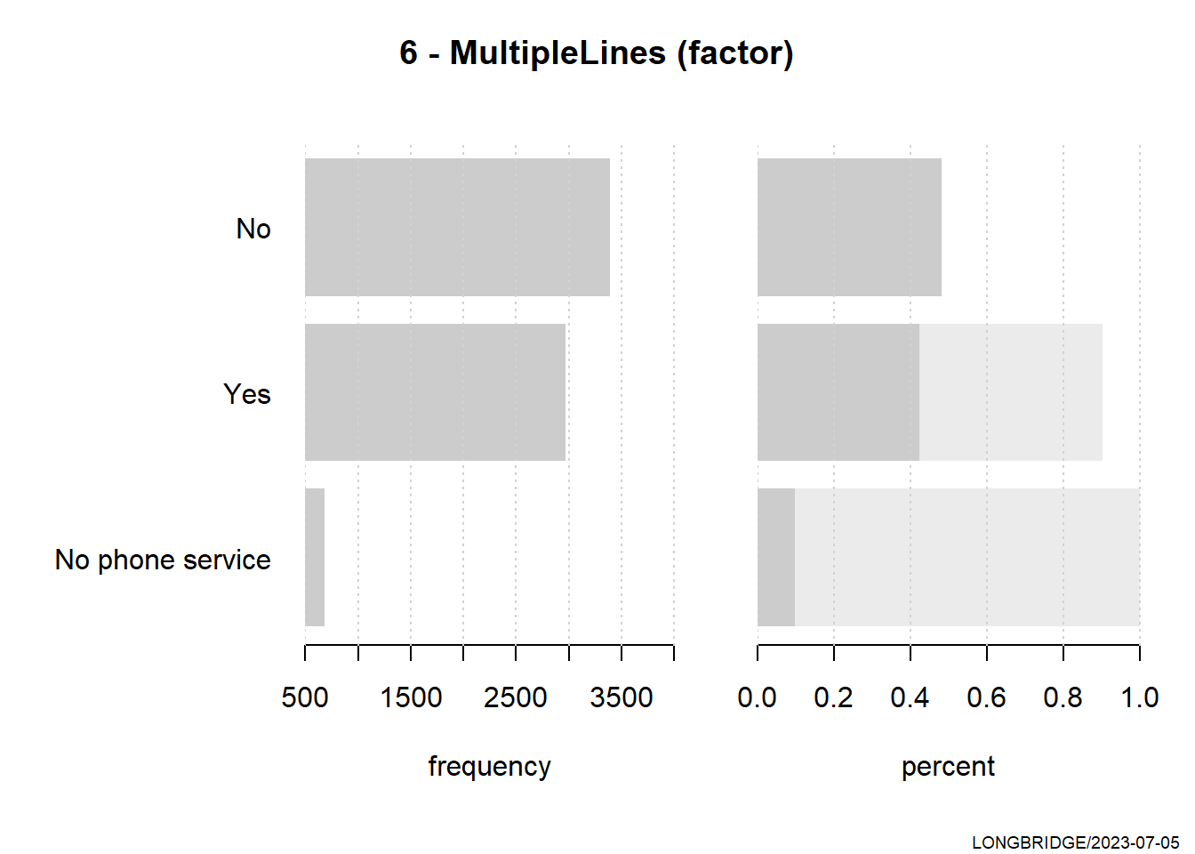

------------------------------------------------------------------------------ 
7 - InternetService (factor)

  length      n    NAs unique levels  dupes
   7'043  7'043      0      3      3      y
         100.0%   0.0%                     

         level   freq   perc  cumfreq  cumperc
1  Fiber optic  3'096  44.0%    3'096    44.0%
2          DSL  2'421  34.4%    5'517    78.3%
3           No  1'526  21.7%    7'043   100.0%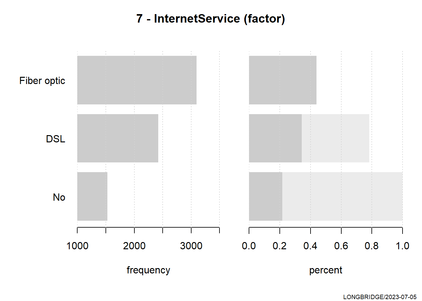

------------------------------------------------------------------------------ 
8 - OnlineSecurity (factor)

  length      n    NAs unique levels  dupes
   7'043  7'043      0      3      3      y
         100.0%   0.0%                     

                 level   freq   perc  cumfreq  cumperc
1                   No  3'498  49.7%    3'498    49.7%
2                  Yes  2'019  28.7%    5'517    78.3%
3  No internet service  1'526  21.7%    7'043   100.0%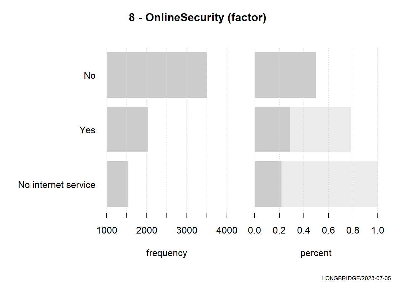

------------------------------------------------------------------------------ 
9 - OnlineBackup (factor)

  length      n    NAs unique levels  dupes
   7'043  7'043      0      3      3      y
         100.0%   0.0%                     

                 level   freq   perc  cumfreq  cumperc
1                   No  3'088  43.8%    3'088    43.8%
2                  Yes  2'429  34.5%    5'517    78.3%
3  No internet service  1'526  21.7%    7'043   100.0%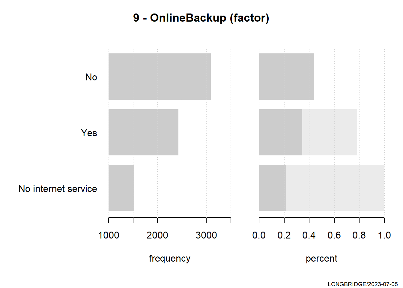

------------------------------------------------------------------------------ 
10 - DeviceProtection (factor)

  length      n    NAs unique levels  dupes
   7'043  7'043      0      3      3      y
         100.0%   0.0%                     

                 level   freq   perc  cumfreq  cumperc
1                   No  3'095  43.9%    3'095    43.9%
2                  Yes  2'422  34.4%    5'517    78.3%
3  No internet service  1'526  21.7%    7'043   100.0%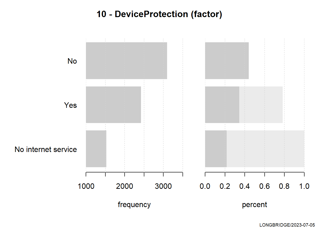

------------------------------------------------------------------------------ 
11 - TechSupport (factor)

  length      n    NAs unique levels  dupes
   7'043  7'043      0      3      3      y
         100.0%   0.0%                     

                 level   freq   perc  cumfreq  cumperc
1                   No  3'473  49.3%    3'473    49.3%
2                  Yes  2'044  29.0%    5'517    78.3%
3  No internet service  1'526  21.7%    7'043   100.0%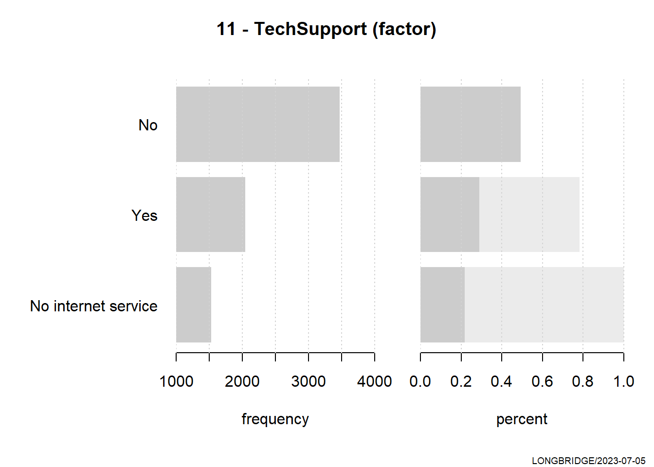

------------------------------------------------------------------------------ 
12 - StreamingTV (factor)

  length      n    NAs unique levels  dupes
   7'043  7'043      0      3      3      y
         100.0%   0.0%                     

                 level   freq   perc  cumfreq  cumperc
1                   No  2'810  39.9%    2'810    39.9%
2                  Yes  2'707  38.4%    5'517    78.3%
3  No internet service  1'526  21.7%    7'043   100.0%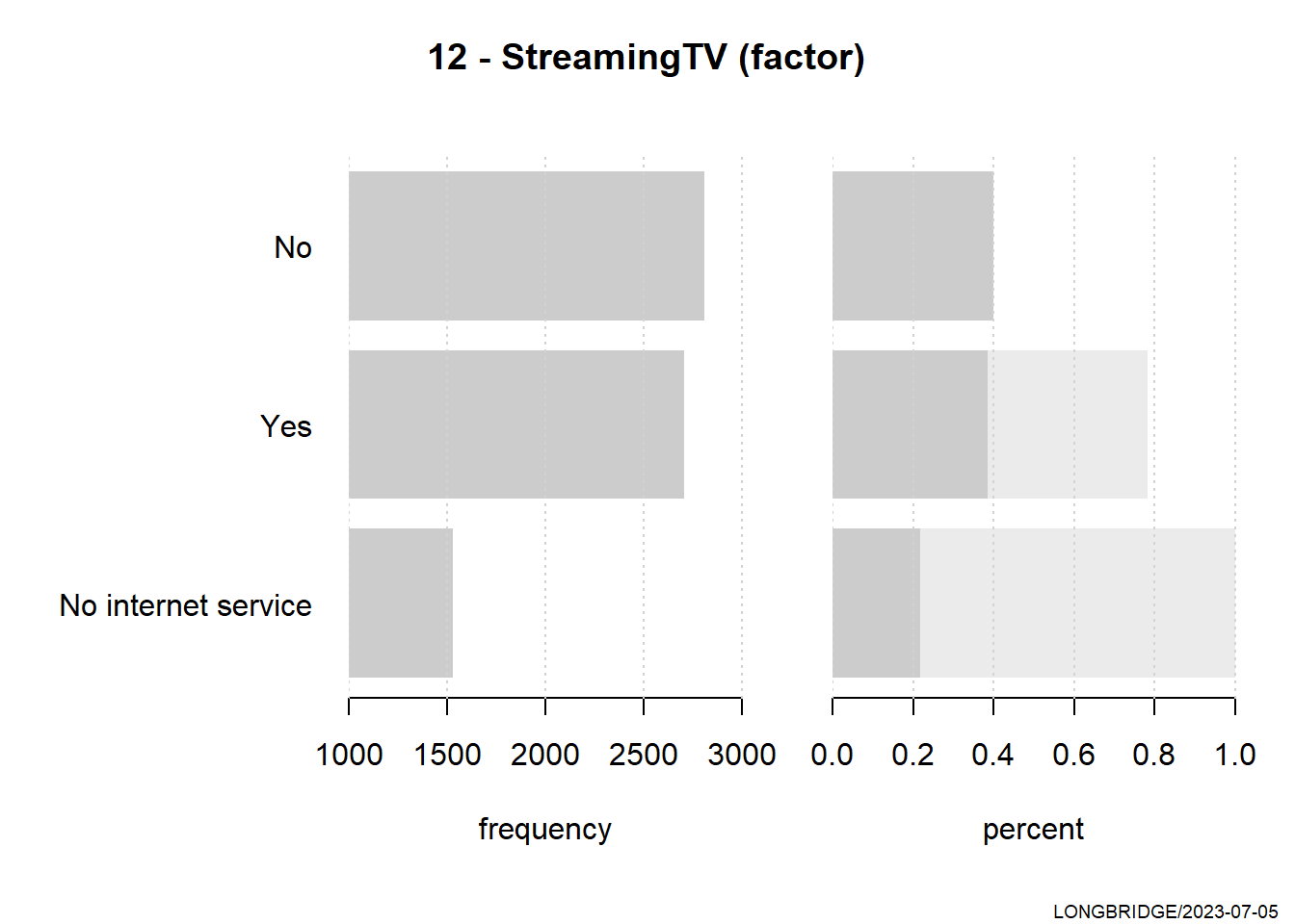

------------------------------------------------------------------------------ 
13 - StreamingMovies (factor)

  length      n    NAs unique levels  dupes
   7'043  7'043      0      3      3      y
         100.0%   0.0%                     

                 level   freq   perc  cumfreq  cumperc
1                   No  2'785  39.5%    2'785    39.5%
2                  Yes  2'732  38.8%    5'517    78.3%
3  No internet service  1'526  21.7%    7'043   100.0%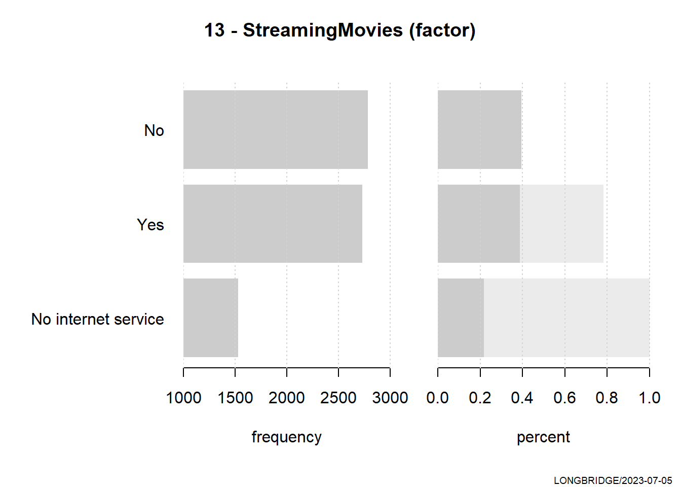

------------------------------------------------------------------------------ 
14 - Contract (factor)

  length      n    NAs unique levels  dupes
   7'043  7'043      0      3      3      y
         100.0%   0.0%                     

            level   freq   perc  cumfreq  cumperc
1  Month-to-month  3'875  55.0%    3'875    55.0%
2        Two year  1'695  24.1%    5'570    79.1%
3        One year  1'473  20.9%    7'043   100.0%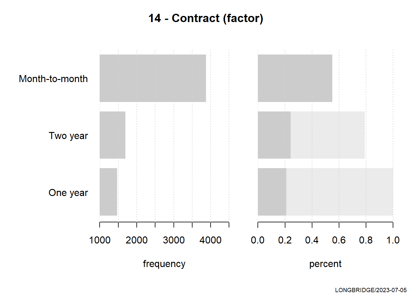

------------------------------------------------------------------------------ 
15 - PaperlessBilling (factor - dichotomous)

  length      n    NAs unique
   7'043  7'043      0      2
         100.0%   0.0%       

      freq   perc  lci.95  uci.95'
No   2'872  40.8%   39.6%   41.9%
Yes  4'171  59.2%   58.1%   60.4%

' 95%-CI (Wilson)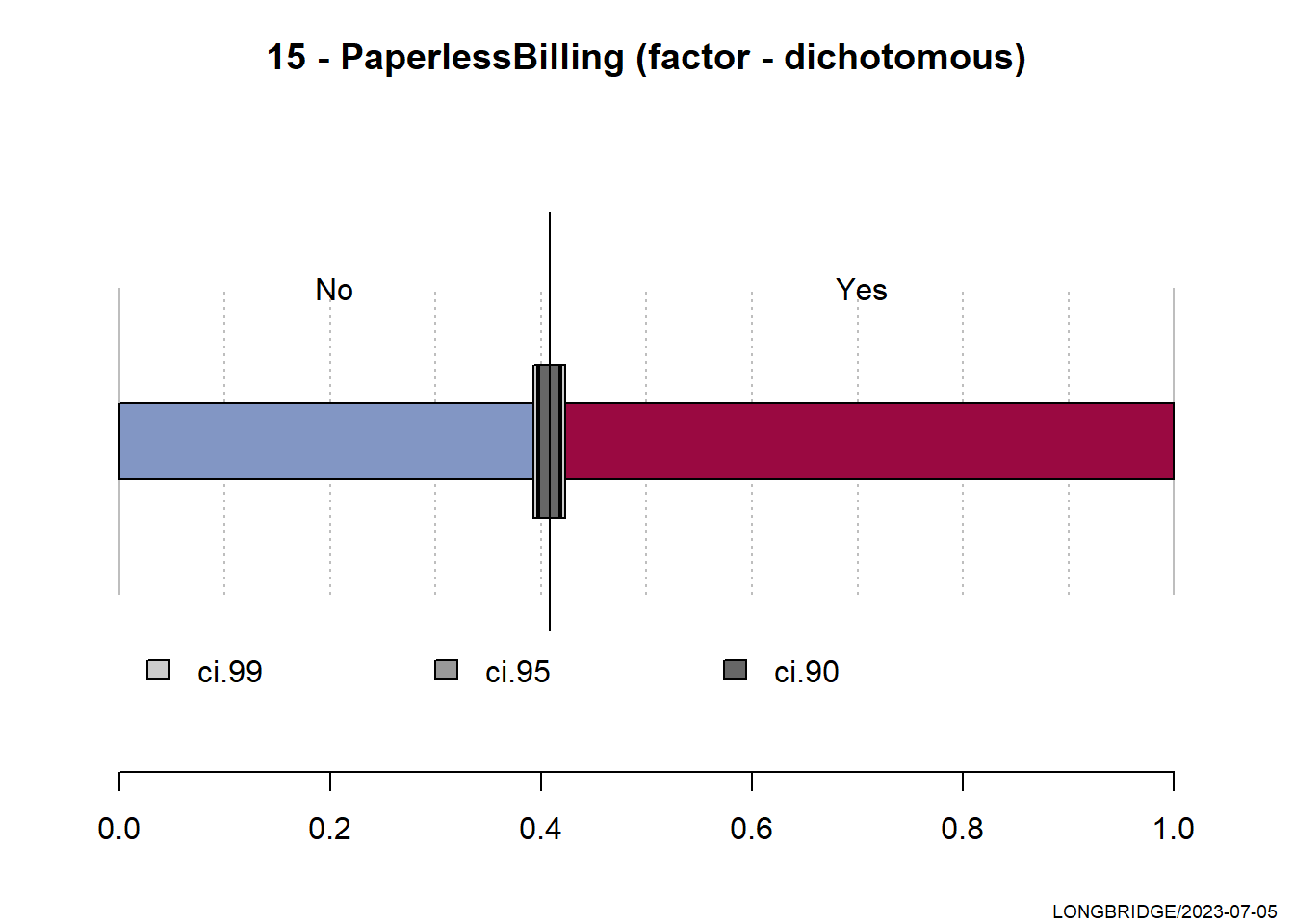

------------------------------------------------------------------------------ 
16 - PaymentMethod (factor)

  length      n    NAs unique levels  dupes
   7'043  7'043      0      4      4      y
         100.0%   0.0%                     

                       level   freq   perc  cumfreq  cumperc
1           Electronic check  2'365  33.6%    2'365    33.6%
2               Mailed check  1'612  22.9%    3'977    56.5%
3  Bank transfer (automatic)  1'544  21.9%    5'521    78.4%
4    Credit card (automatic)  1'522  21.6%    7'043   100.0%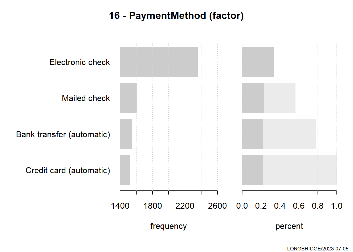

------------------------------------------------------------------------------ 
17 - Churn (factor - dichotomous)

  length      n    NAs unique
   7'043  7'043      0      2
         100.0%   0.0%       

      freq   perc  lci.95  uci.95'
No   5'174  73.5%   72.4%   74.5%
Yes  1'869  26.5%   25.5%   27.6%

' 95%-CI (Wilson)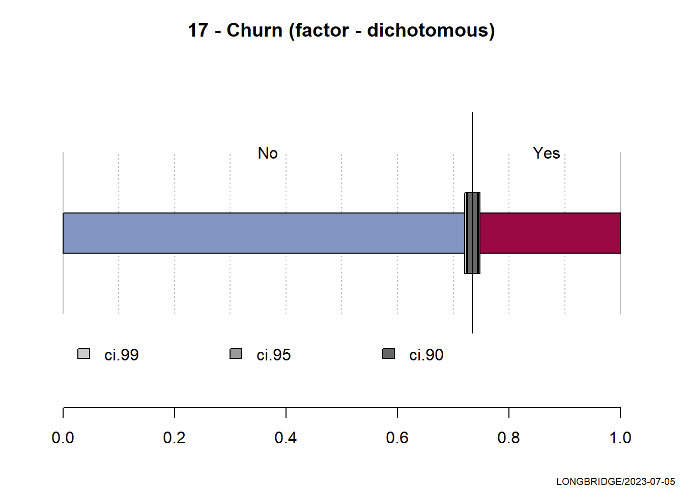

Code

# Gender Distribution

telco_df %>% 
  group_by(gender) %>%
  summarise(Freq = n()) %>% 
  mutate(prop = Freq/sum(Freq)) %>% 
  filter(Freq != 0) %>% 
  
  ggplot(mapping = aes(x = 2, y = prop, fill = gender))+
  geom_bar(width = 1, color = "white", stat = "identity") +
  xlim(0.5, 2.5) +
  coord_polar(theta = "y", start = 0) +
  theme_void() +
  scale_y_continuous(labels = scales::percent) +
  geom_text(aes(label = paste0(round(prop*100, 1), "%")), size = 4, position = position_stack(vjust = 0.5)) +
  scale_fill_manual(values = c("#fc0394","#03adfc")) +
  #theme(axis.text.x = element_text(angle = 90), legend.position = "top")+
  labs(title = "Customer Distribution by Gender",
       x = "",
       y = "",
       fill = "") +
  theme(legend.position = "top") +
   theme(title = element_text(family = "Sans", face = "bold", size = 16))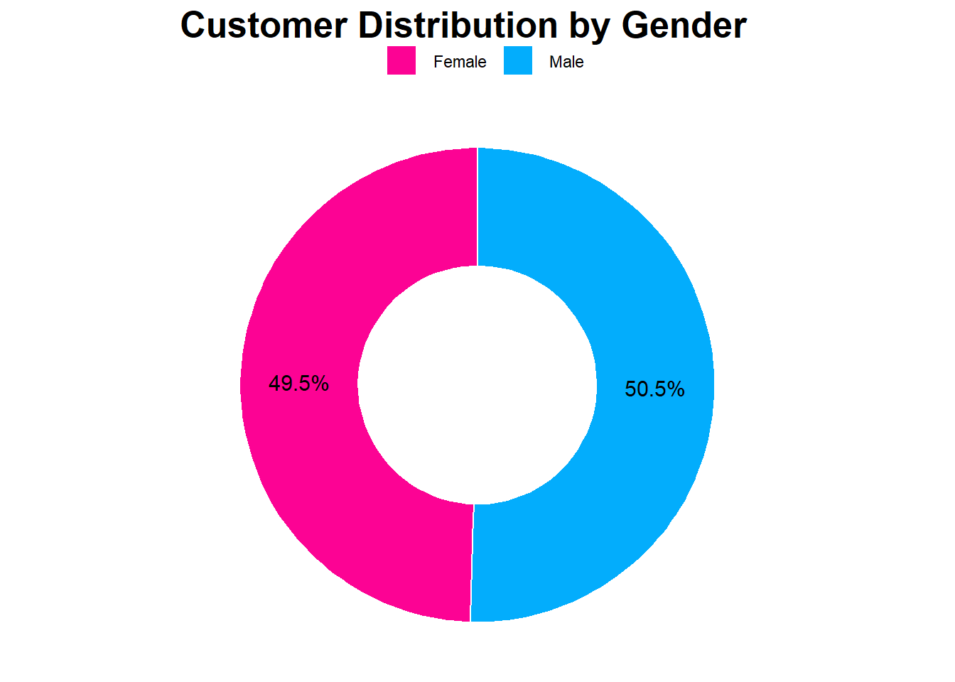

Code

# Distribution of Churned Customer


telco_df %>% 
  mutate(Churn = case_when(Churn == "No" ~ "Not Churned",
                            TRUE ~ "Churned")) %>% 
  group_by(Churn) %>%
  summarise(Freq = n()) %>% 
  mutate(prop = Freq/sum(Freq)) %>% 
  filter(Freq != 0) %>% 
  
  ggplot(mapping = aes(x = 2, y = prop, fill = Churn))+
  geom_bar(width = 1, color = "white", stat = "identity") +
  xlim(0.5, 2.5) +
  coord_polar(theta = "y", start = 0) +
  theme_void() +
  scale_y_continuous(labels = scales::percent) +
  geom_text(aes(label = paste0(round(prop*100, 1), "%")), size = 4, position = position_stack(vjust = 0.5)) +
  scale_fill_manual(values = c('#FF0000', '#0000FF')) +
  #theme(axis.text.x = element_text(angle = 90), legend.position = "top")+
  labs(title = 'Distribution of Churned Customer',
       x = "",
       y = "",
       fill = "") +
  theme(legend.position = "top") +
   theme(title = element_text(family = "Sans", face = "bold", size = 16))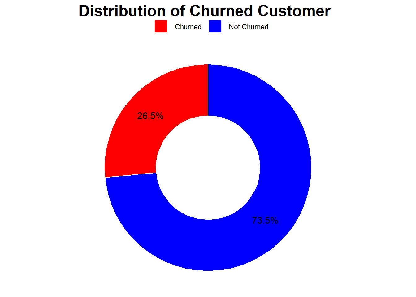

Code

# Payment Methods used by Customer


telco_df %>% 
  group_by(PaymentMethod) %>% 
  summarise(Count = n()) %>% 
  ggplot(aes(x = reorder(PaymentMethod, Count), y = Count)) +
  geom_bar(stat = "identity", width = 0.3, fill = "steelblue", color = "white") +
  labs(title = 'Payment Methods used by Customer',
       x = "Payment Method") +
  theme(title = element_text(family = "Sans", face = "bold", size = 16),
        axis.title = element_text(family = "sans", size = 10, face = "plain")) +
  theme_clean() +
  scale_y_continuous(labels = scales::comma) +
  geom_text(aes(label = Count), size = 3.5)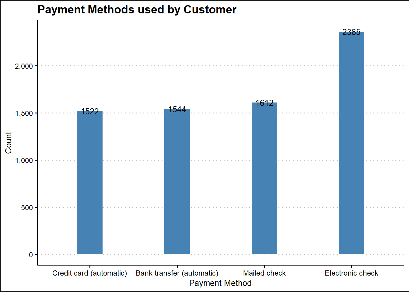

Code

# Distribution of Customers by Internet Service

telco_df %>% 
  group_by(InternetService) %>% 
  summarise(Count = n()) %>% 
  ggplot(aes(x = reorder(InternetService, Count), y = Count)) +
  geom_bar(stat = "identity", width = 0.3, fill = "steelblue", color = "white") +
  labs(title = 'Distribution of Customers by Internet Service',
       x = "Internet Service") +
  theme(title = element_text(family = "Sans", face = "bold", size = 16),
        axis.title = element_text(family = "sans", size = 10, face = "plain")) +
  theme_clean() +
  scale_y_continuous(labels = scales::comma) +
  geom_text(aes(label = Count), size = 3.5)

Code

# Distribution of Customer by Phone service

telco_df %>% 
  group_by(PhoneService) %>%
  summarise(Freq = n()) %>% 
  mutate(prop = Freq/sum(Freq)) %>% 
  filter(Freq != 0) %>% 
  
  ggplot(mapping = aes(x = 2, y = prop, fill = PhoneService))+
  geom_bar(width = 1, color = "white", stat = "identity") +
  xlim(0.5, 2.5) +
  coord_polar(theta = "y", start = 0) +
  theme_void() +
  scale_y_continuous(labels = scales::percent) +
  geom_text(aes(label = paste0(round(prop*100, 1), "%")), size = 4, position = position_stack(vjust = 0.5)) +
  scale_fill_manual(values = c('#FF0000', '#0000FF')) +
  #theme(axis.text.x = element_text(angle = 90), legend.position = "top")+
  labs(title = 'Distribution of Customer by \nPhone Service',
       x = "",
       y = "",
       fill = "") +
  theme(legend.position = "top") +
   theme(title = element_text(family = "Sans", face = "bold", size = 16))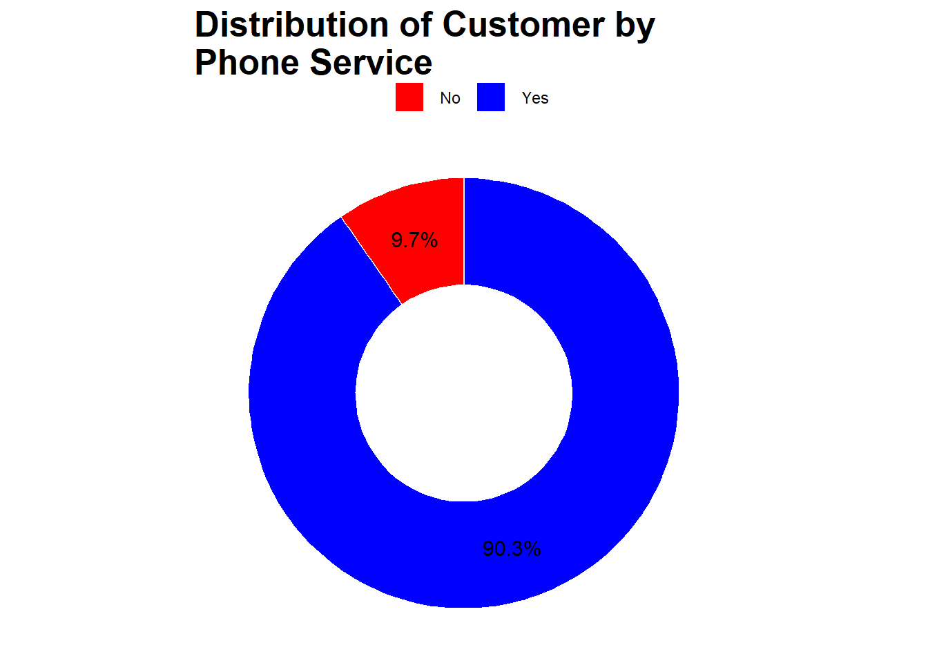

Code

# Distribution of Customer by Paperless Billing

telco_df %>% 
  group_by(PaperlessBilling) %>%
  summarise(Freq = n()) %>% 
  mutate(prop = Freq/sum(Freq)) %>% 
  filter(Freq != 0) %>% 
  
  ggplot(mapping = aes(x = 2, y = prop, fill = PaperlessBilling))+
  geom_bar(width = 1, color = "white", stat = "identity") +
  xlim(0.5, 2.5) +
  coord_polar(theta = "y", start = 0) +
  theme_void() +
  scale_y_continuous(labels = scales::percent) +
  geom_text(aes(label = paste0(round(prop*100, 1), "%")), size = 4, position = position_stack(vjust = 0.5)) +
  scale_fill_manual(values = c('#FF0000', '#0000FF')) +
  #theme(axis.text.x = element_text(angle = 90), legend.position = "top")+
  labs(title = 'Distribution of Customer by \nPaperless Billing',
       x = "",
       y = "",
       fill = "") +
  theme(legend.position = "top") +
   theme(title = element_text(family = "Sans", face = "bold", size = 16))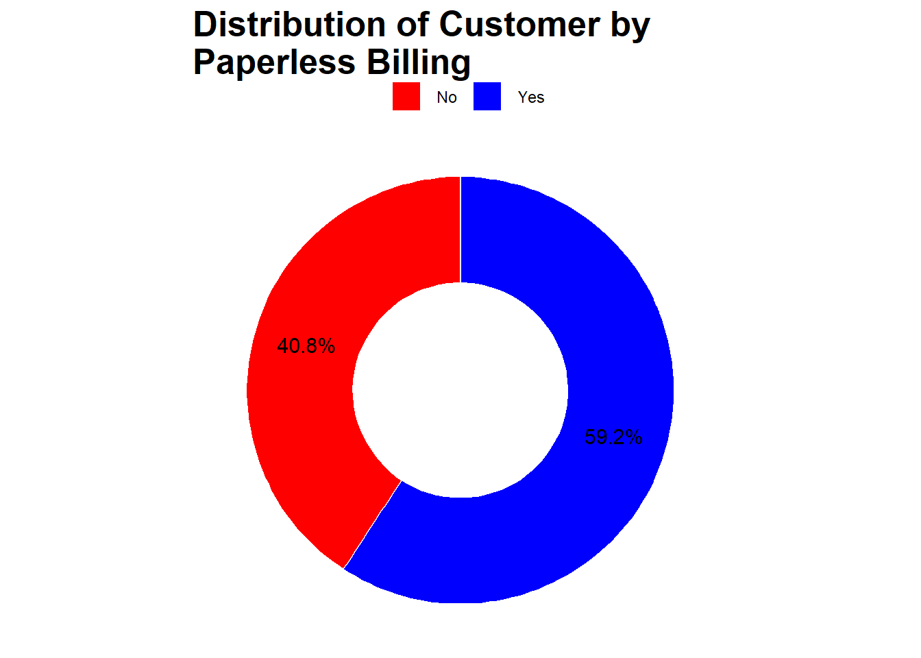

Code

# Distribution of Customers by Contract

telco_df %>% 
  group_by(Contract) %>% 
  summarise(Count = n()) %>% 
  ggplot(aes(x = reorder(Contract, Count), y = Count)) +
  geom_bar(stat = "identity", width = 0.3, fill = "steelblue", color = "white") +
  labs(title = 'Distribution of Customers by Contract',
       x = "Contract Type") +
  theme(title = element_text(family = "Sans", face = "bold", size = 16),
        axis.title = element_text(family = "sans", size = 10, face = "plain")) +
  theme_clean() +
  scale_y_continuous(labels = scales::comma) +
  geom_text(aes(label = Count), size = 3.5)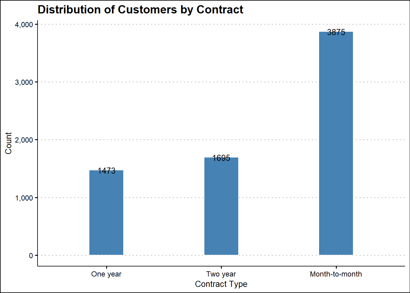

Code

# Distribution of Customer by Online Security

telco_df %>% 
  group_by(OnlineSecurity) %>%
  summarise(Freq = n()) %>% 
  mutate(prop = Freq/sum(Freq)) %>% 
  filter(Freq != 0) %>% 
  
  ggplot(mapping = aes(x = 2, y = prop, fill = OnlineSecurity))+
  geom_bar(width = 1, color = "white", stat = "identity") +
  xlim(0.5, 2.5) +
  coord_polar(theta = "y", start = 0) +
  theme_void() +
  scale_y_continuous(labels = scales::percent) +
  geom_text(aes(label = paste0(round(prop*100, 1), "%")), size = 4, position = position_stack(vjust = 0.5)) +
  scale_fill_manual(values = c('#FF0000', 'tomato', 'darkorange')) +
  #theme(axis.text.x = element_text(angle = 90), legend.position = "top")+
  labs(title = 'Distribution of Customer by \nOnline Security',
       x = "",
       y = "",
       fill = "") +
  theme(legend.position = "top") +
   theme(title = element_text(family = "Sans", face = "bold", size = 16))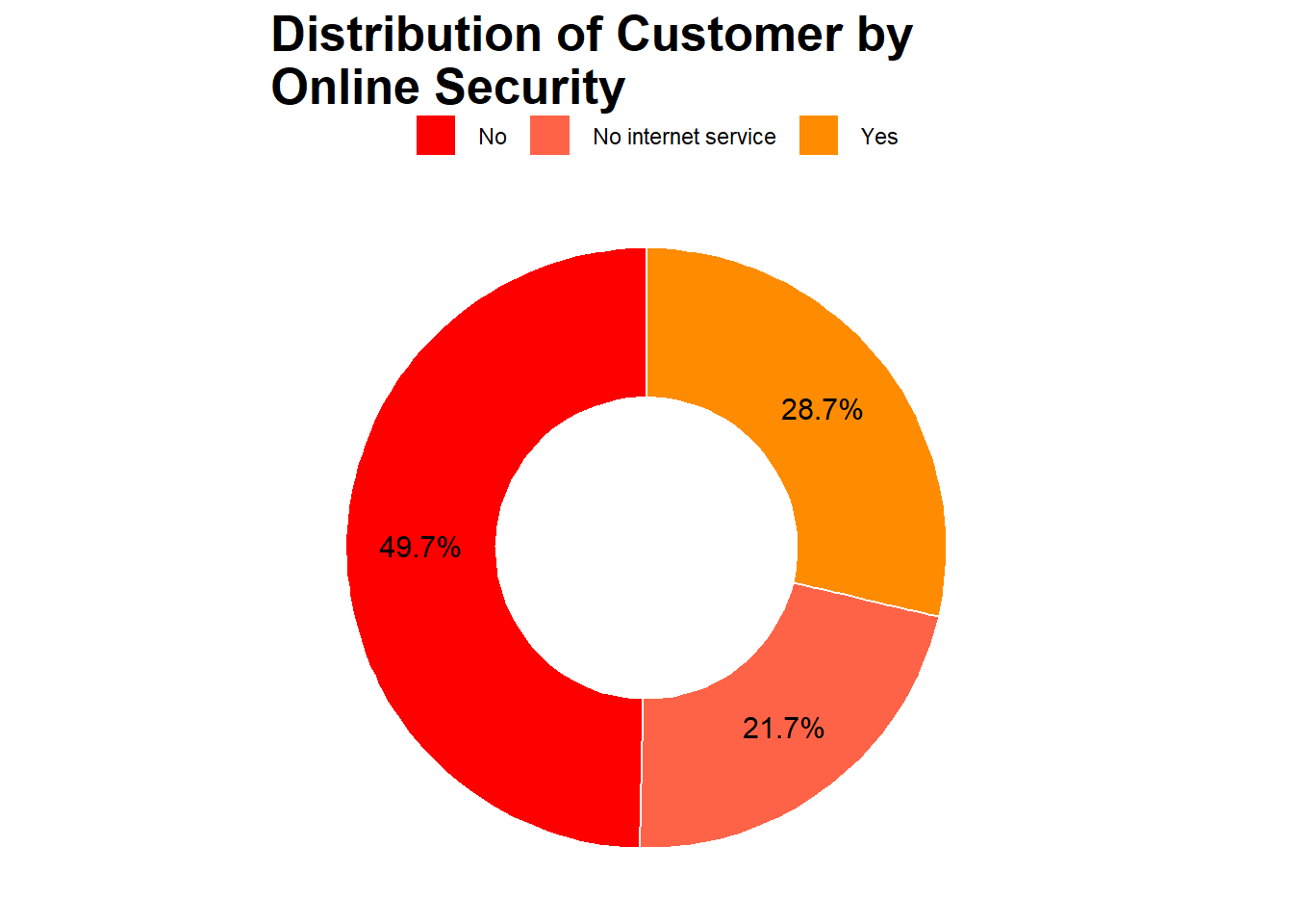

Code

# Proportion of Churn by Gender


telco_df %>% 
  mutate(Churn = case_when(Churn == "No" ~ "Not Churned",
                            TRUE ~ "Churned")) %>% 
  group_by(gender, Churn) %>%
  summarise(Count = n()) %>% 
  mutate(Prop = Count/sum(Count)) %>% 
  ggplot(aes(x = reorder(gender, Prop), y = Prop, fill = Churn)) +
  geom_bar(stat = "identity", width = 0.3, color = "white", position = "fill") +
  labs(title = 'Proportion of Churn by Gender',
       x = "",
       y = "") +
   scale_fill_manual(values = c('#FF0000', '#0000FF')) +
  theme(title = element_text(family = "Sans", face = "bold", size = 16),
        axis.title = element_text(family = "sans", size = 10, face = "plain")) +
  theme_clean() +
  scale_y_continuous(labels = scales::percent) +
  geom_text(aes(label = paste0(round(Prop*100,1),"%")), size = 3.5, position = position_fill(vjust = 0.5))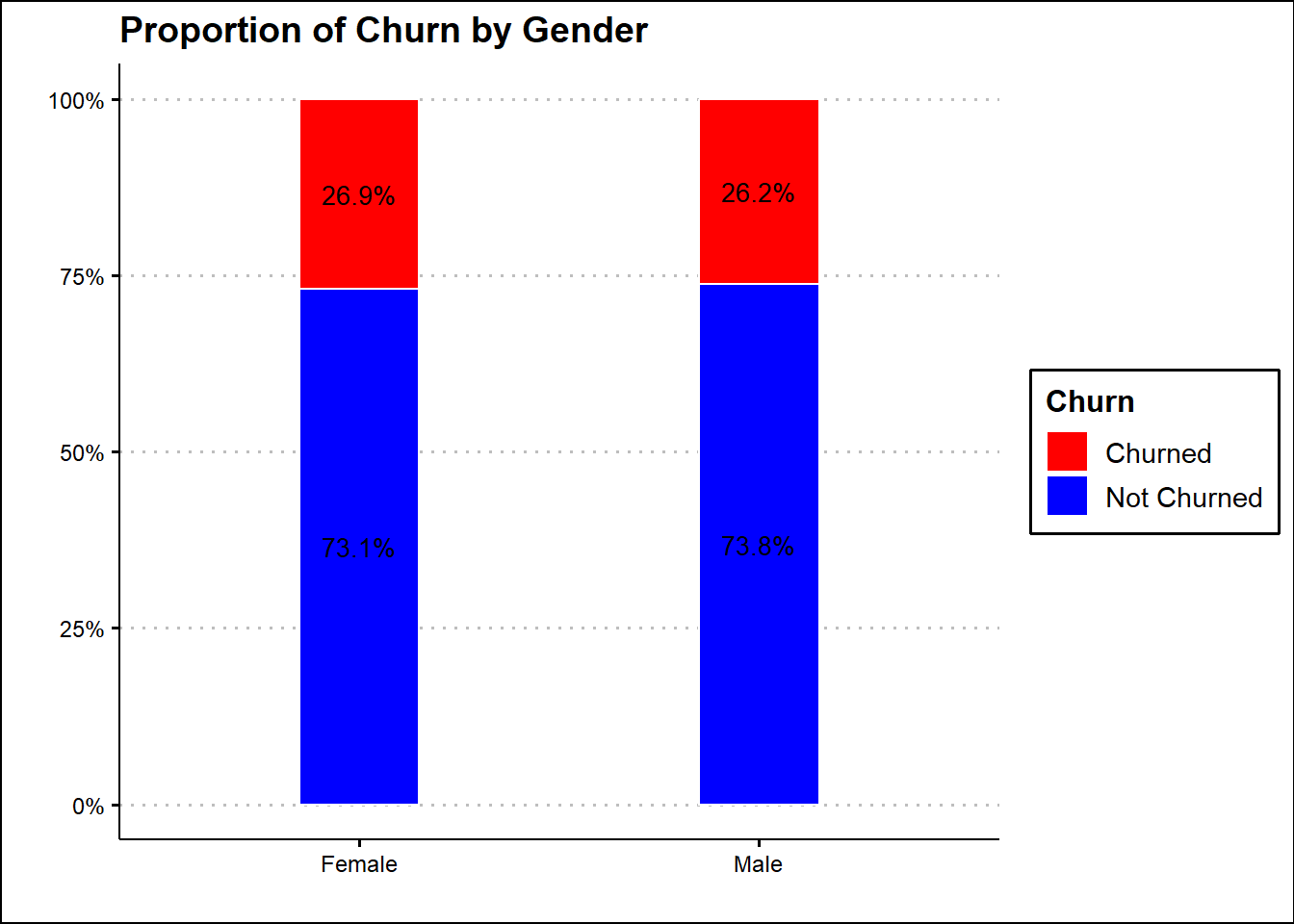

Code

# Proportion of Churn by PaymentMethod


telco_df %>% 
  mutate(Churn = case_when(Churn == "No" ~ "Not Churned",
                            TRUE ~ "Churned")) %>% 
  group_by(PaymentMethod, Churn) %>%
  summarise(Count = n()) %>% 
  mutate(Prop = Count/sum(Count)) %>% 
  ggplot(aes(x = reorder(PaymentMethod, Prop), y = Prop, fill = Churn)) +
  geom_bar(stat = "identity", width = 0.5, color = "white", position = "fill") +
  labs(title = 'Proportion of Churn by Payment Method',
       x = "",
       y = "") +
   scale_fill_manual(values = c('#FF0000', '#0000FF')) +
  theme(title = element_text(family = "Sans", face = "bold", size = 16),
        axis.title = element_text(family = "sans", size = 10, face = "plain")) +
  theme_clean() +
  scale_y_continuous(labels = scales::percent) +
  geom_text(aes(label = paste0(round(Prop*100,1),"%")), size = 3.5, position = position_fill(vjust = 0.5))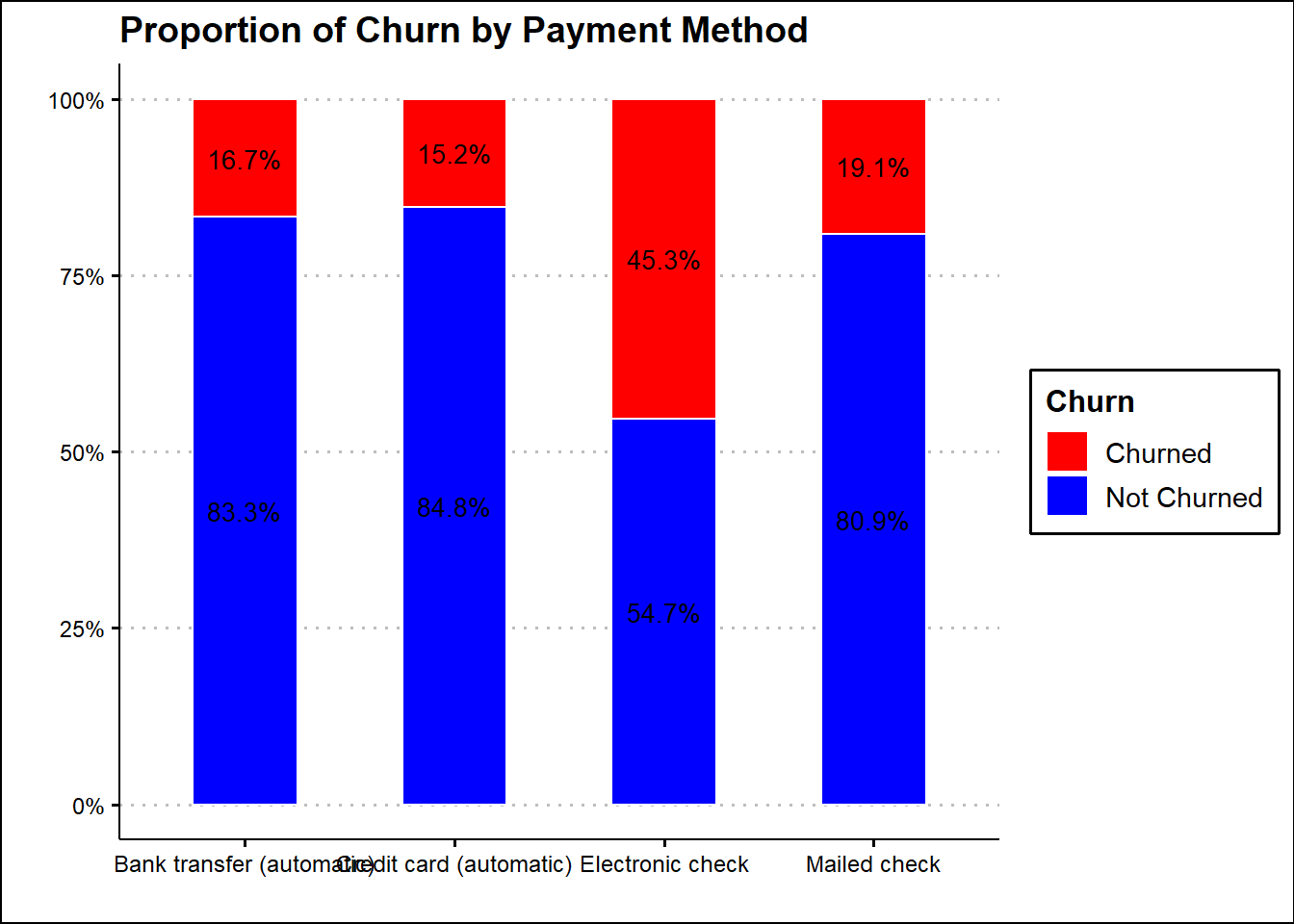

Code

# Proportion of Churn by Contract Type


telco_df %>% 
  mutate(Churn = case_when(Churn == "No" ~ "Not Churned",
                            TRUE ~ "Churned")) %>% 
  group_by(Contract, Churn) %>%
  summarise(Count = n()) %>% 
  mutate(Prop = Count/sum(Count)) %>% 
  ggplot(aes(x = reorder(Contract, Prop), y = Prop, fill = Churn)) +
  geom_bar(stat = "identity", width = 0.5, color = "white", position = "fill") +
  labs(title = 'Proportion of Churn by Contract Type',
       x = "",
       y = "") +
   scale_fill_manual(values = c('#FF0000', '#0000FF')) +
  theme(title = element_text(family = "Sans", face = "bold", size = 16),
        axis.title = element_text(family = "sans", size = 10, face = "plain")) +
  theme_clean() +
  scale_y_continuous(labels = scales::percent) +
  geom_text(aes(label = paste0(round(Prop*100,1),"%")), size = 3.5, position = position_fill(vjust = 0.5))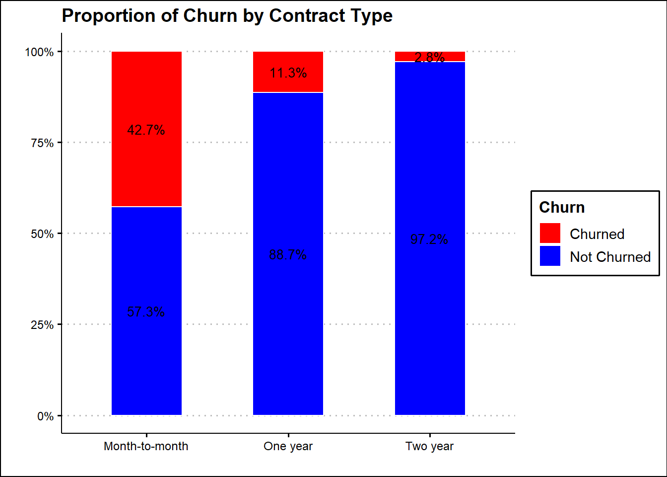

Modelling

Data Quality

Check dataframe for NAs

Code

any(is.na(telco_df))

[1] FALSE

No NA is found. The dataset is complete without any missing values.

Code

# split data to train and test set

set.seed(1234)

split <- telco_df %>% 
  select(-customerID) %>% 
  initial_split(prop = 0.75, strata = Churn) # 75% training set | 25% testing set

df_train <- split %>% 
  training()

df_test <- split %>% 
  testing()

Model Recipe

Code

rec <- recipe(Churn ~ ., data = df_train)

# add preprocessing

prepro <- rec %>% 
  step_dummy(all_nominal_predictors()) %>% 
  step_other(all_nominal_predictors()) %>% 
  step_filter_missing(all_nominal_predictors(),threshold = 0) %>% 
  prep()

prepro

Define the model with parsnip

Code

## Logistic Regression

lr <- logistic_reg(
  mode = "classification"
) %>% 
  set_engine("glm")


## Nearest Neighbor

knn <- nearest_neighbor(
  mode = "classification"
) %>% 
  set_engine("kknn")

## Random Forest

rf <- rand_forest(mode = "classification") %>% 
  set_engine("ranger", importance='impurity')

## Gradient Boost

gb <- boost_tree(mode = "classification") %>% 
  set_engine("xgboost")

Define models workflow

Code

## Logistic Regression

lr_wf <- workflow() %>% 
  add_recipe(prepro) %>% 
  add_model(lr)


## Nearest Neighbor

knn_wf <- workflow() %>% 
  add_recipe(prepro) %>% 
  add_model(knn)

## Random Forest

rf_wf <- workflow() %>% 
  add_recipe(prepro) %>% 
  add_model(rf)


## Gradient Boost

gb_wf <- workflow() %>% 
  add_recipe(prepro) %>% 
  add_model(gb)

Obtaining Predictions

Code

set.seed(1234)

## Logistic Regression

lr_pred <- lr_wf %>% 
  fit(df_train) %>% 
  predict(df_test) %>% 
  bind_cols(df_test)


## Nearest Neighbor

knn_pred <- knn_wf %>% 
  fit(df_train) %>% 
  predict(df_test) %>% 
  bind_cols(df_test)

## Random Forest

rf_pred <- rf_wf %>% 
  fit(df_train) %>% 
  predict(df_test) %>% 
  bind_cols(df_test)


## Gradient Boost

gb_pred <- gb_wf %>% 
  fit(df_train) %>% 
  predict(df_test) %>% 
  bind_cols(df_test)

Evaluating model performance

kap: Kappa
sens: Sensitivity
spec: Specificity
f_meas: F1
mcc: Matthews correlation coefficient

Logistic Regression

Code

lr_pred %>% 
  conf_mat(truth = Churn, estimate = .pred_class) %>% 
  summary()

# A tibble: 13 x 3
   .metric              .estimator .estimate
   <chr>                <chr>          <dbl>
 1 accuracy             binary         0.786
 2 kap                  binary         0.410
 3 sens                 binary         0.894
 4 spec                 binary         0.487
 5 ppv                  binary         0.828
 6 npv                  binary         0.625
 7 mcc                  binary         0.416
 8 j_index              binary         0.381
 9 bal_accuracy         binary         0.691
10 detection_prevalence binary         0.793
11 precision            binary         0.828
12 recall               binary         0.894
13 f_meas               binary         0.860

Nearest Neighbor

Code

knn_pred %>% 
  conf_mat(truth = Churn, estimate = .pred_class) %>% 
  summary()

# A tibble: 13 x 3
   .metric              .estimator .estimate
   <chr>                <chr>          <dbl>
 1 accuracy             binary         0.708
 2 kap                  binary         0.122
 3 sens                 binary         0.884
 4 spec                 binary         0.220
 5 ppv                  binary         0.758
 6 npv                  binary         0.407
 7 mcc                  binary         0.131
 8 j_index              binary         0.104
 9 bal_accuracy         binary         0.552
10 detection_prevalence binary         0.856
11 precision            binary         0.758
12 recall               binary         0.884
13 f_meas               binary         0.816

Random Forest

Code

rf_pred %>% 
  conf_mat(truth = Churn, estimate = .pred_class) %>% 
  summary()

# A tibble: 13 x 3
   .metric              .estimator .estimate
   <chr>                <chr>          <dbl>
 1 accuracy             binary         0.780
 2 kap                  binary         0.369
 3 sens                 binary         0.911
 4 spec                 binary         0.419
 5 ppv                  binary         0.813
 6 npv                  binary         0.630
 7 mcc                  binary         0.382
 8 j_index              binary         0.330
 9 bal_accuracy         binary         0.665
10 detection_prevalence binary         0.823
11 precision            binary         0.813
12 recall               binary         0.911
13 f_meas               binary         0.859

Gradient Boost

Code

gb_pred %>% 
  conf_mat(truth = Churn, estimate = .pred_class) %>% 
  summary()

# A tibble: 13 x 3
   .metric              .estimator .estimate
   <chr>                <chr>          <dbl>
 1 accuracy             binary         0.774
 2 kap                  binary         0.367
 3 sens                 binary         0.895
 4 spec                 binary         0.440
 5 ppv                  binary         0.815
 6 npv                  binary         0.602
 7 mcc                  binary         0.374
 8 j_index              binary         0.335
 9 bal_accuracy         binary         0.668
10 detection_prevalence binary         0.806
11 precision            binary         0.815
12 recall               binary         0.895
13 f_meas               binary         0.853

The random forest seems to be better off going by the sensitivity and the specificity metrics.

Random Forest Roc Curve

Code

## Random Forest

prob_preds <- rf_wf %>% 
  fit(df_train) %>% 
  predict(df_test, type = "prob") %>% 
  bind_cols(df_test)


threshold_df <- prob_preds %>% 
  roc_curve(truth = Churn, estimate = .pred_No)

threshold_df %>% 
  autoplot()

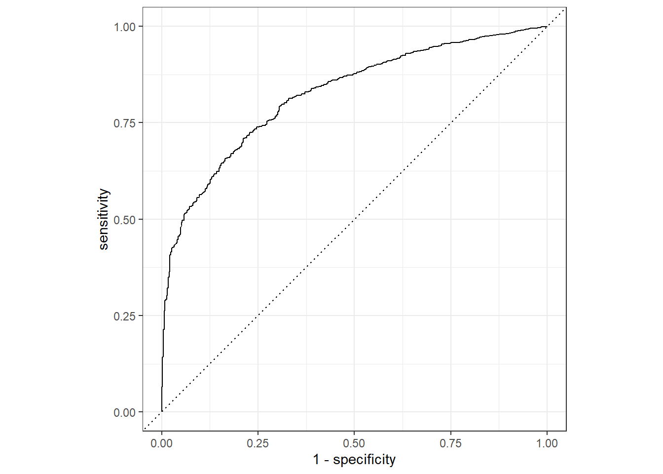
Code

roc_auc(prob_preds, truth = Churn, estimate = .pred_No)

# A tibble: 1 x 3
  .metric .estimator .estimate
  <chr>   <chr>          <dbl>
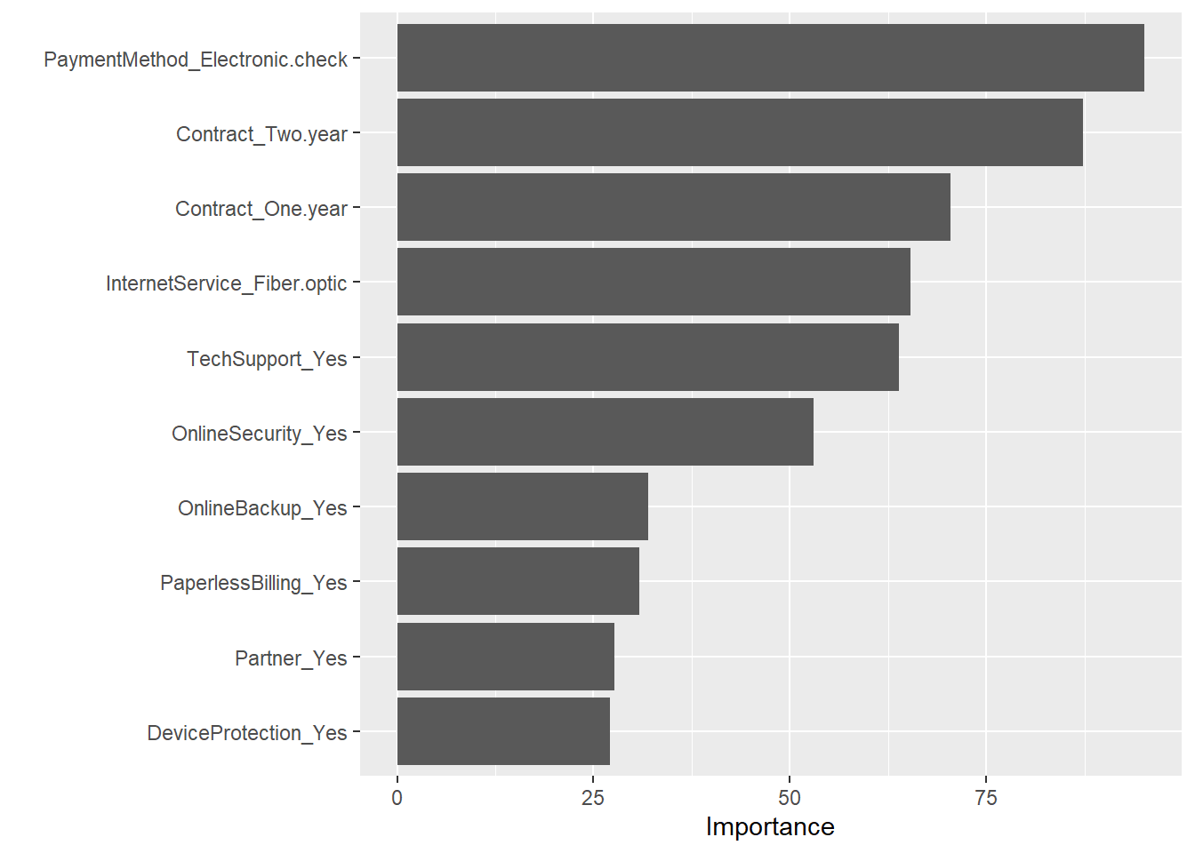
1 roc_auc binary         0.824

Variable Importance Plot

Relative variable importance plot

Code

final_rf_model <-
  rf_wf %>%
  fit(data = df_train)

final_rf_model

== Workflow [trained] ==========================================================
Preprocessor: Recipe
Model: rand_forest()

-- Preprocessor ----------------------------------------------------------------
3 Recipe Steps

* step_dummy()
* step_other()
* step_filter_missing()

-- Model -----------------------------------------------------------------------
Ranger result

Call:
 ranger::ranger(x = maybe_data_frame(x), y = y, importance = ~"impurity",      num.threads = 1, verbose = FALSE, seed = sample.int(10^5,          1), probability = TRUE) 

Type:                             Probability estimation 
Number of trees:                  500 
Sample size:                      5281 
Number of independent variables:  26 
Mtry:                             5 
Target node size:                 10 
Variable importance mode:         impurity 
Splitrule:                        gini 
OOB prediction error (Brier s.):  0.1469603

Code

final_rf_model %>% 
  pull_workflow_fit()

parsnip model object

Ranger result

Call:
 ranger::ranger(x = maybe_data_frame(x), y = y, importance = ~"impurity",      num.threads = 1, verbose = FALSE, seed = sample.int(10^5,          1), probability = TRUE) 

Type:                             Probability estimation 
Number of trees:                  500 
Sample size:                      5281 
Number of independent variables:  26 
Mtry:                             5 
Target node size:                 10 
Variable importance mode:         impurity 
Splitrule:                        gini 
OOB prediction error (Brier s.):  0.1469603

Code

## variable importance plot

library(vip)

final_rf_model %>%
  extract_fit_parsnip() %>%
  vip()